
By Guillaume Bertrand
I started astronomy at the age of 15, in 2003, with the opposition of Mars. I quickly joined the astronomy club “Village du ciel” based in Vendée to exchange with other amateur astronomers. My first instrument was a 114/900, I got all the planetary imaging I could from it. Those were the days of the modified Vesta Pro webcams. I used this 114/900 intensively for 5 years with a systematic sharing of my observations with the planetary observations commission of the SAF. In parallel, from 2005 to 2009 I developed and maintained the planetary ephemeris calculation software AstroCalc. This exercise allowed me to self-train in software and web development in several languages and to make it my job. A little less active afterwards because of professional, family and musical life (I am also a musician), but still imaging and planetary tracking in the background with a 254mm dobson. I took a turn in 2018 by deciding to build myself an instrument (400mm dobson compact) dedicated only to visual and drawing. I get a lot of pleasure out of trying to find the smallest photon on very weak objects and putting the result on paper. At the end of 2021, I discovered the very ingenious Sol’ex/Star’ex project initiated by Christian Buil. I quickly decided to invest in the subject with the idea of getting serious about spectro afterwards. Everything is going very fast, the first results give me the shivers! I read a lot about it… in short… the spectro absorbs me! Being able to repeat pro observations with minimal hardware configurations or even better collaborate on pro-am projects is highly motivating.
This study demonstrates that it is possible to detect and study the magnetic field of a star with a 0.072m telescope, a polarimeter made from 3D cinema glasses and a spectrograph made from 3D printing. The chosen target is α2 CVn, an Ap-type (chemically peculiar) star widely studied for its magnetic field and variability. In order to obtain a complete coverage according to the phase, 10 nights of observations were necessary. The Star’Ex spectrograph equipped with a 2400 line/mm grating and a 10μm slit coupled with a 72mm f/6 refractor delivers spectra with an average resolution of 25000. We will rely on the Zeeman effect and calculate the Stokes I and V profiles on the Hα line to extract the information of interest.
Introduction
In November 2018, I came out of a lecture given by Christian Buil at the Sky and Space meetings very impressed. This conference was entitled “Spectrography: the new horizons”. I learned, among other things, that spectropolarimetry was on the way to becoming accessible to amateurs and would make it possible to measure and map the magnetic field of stars. Fascinating field of investigation… but at the time it seemed far from my possibilities!
Since then, years have passed and the amazing Star’Ex spectrograph made with a 3D printer has appeared, making it possible to make high resolution spectra of very good quality. In parallel, the field of possibilities with the Sol’Ex project (solar counterpart of Star’Ex) has evolved and it is now possible to produce magnetograms using a polarimeter made from 3D cinema glasses.
I thought it would be great to adapt this little polarimeter for stars and try to detect the polarisation of the bright star α2 CVn (Cor Caroli) located about 110 light years away. It is the first star classified with the chemically peculiar ‘Ap’ type, which has been the subject of much study regarding its variability and magnetic field.
The challenge for me was to confirm the detection with a modest hardware configuration, accessible to all: a SkyWatcher 72mm scope on a Heq5 mount associated with the Star’Ex spectrograph.
Méthodology
The measurement of the magnetic field of a star is made possible by the Zeeman effect. This quantum effect shows that within a spectrum, certain “magnetically sensitive” lines will split into several components in the presence of a magnetic field. These components are circularly polarised for the longitudinal field (in the viewing axis) and linearly polarised (perpendicular to the viewing axis) for the transverse field. The sensitivity of the line to the magnetic field is defined by the Landé factor between 0 and 3. To get a better idea of the phenomenon, here is a short video from ESO offering a visual representation of the Zeeman effect:
The polarimeter built for the Sol’Ex allows us to isolate the left (-45°) and right (+45°) circular polarisation. It therefore allows us to measure the longitudinal magnetic field.
Left and right polarisation animation highlighting the Zeeman effect during the passage of sunspot AR 3004. Slightly to the right of centre: Fe I 6173 A ray. Sol’Ex + SW72ED f/6 refractor
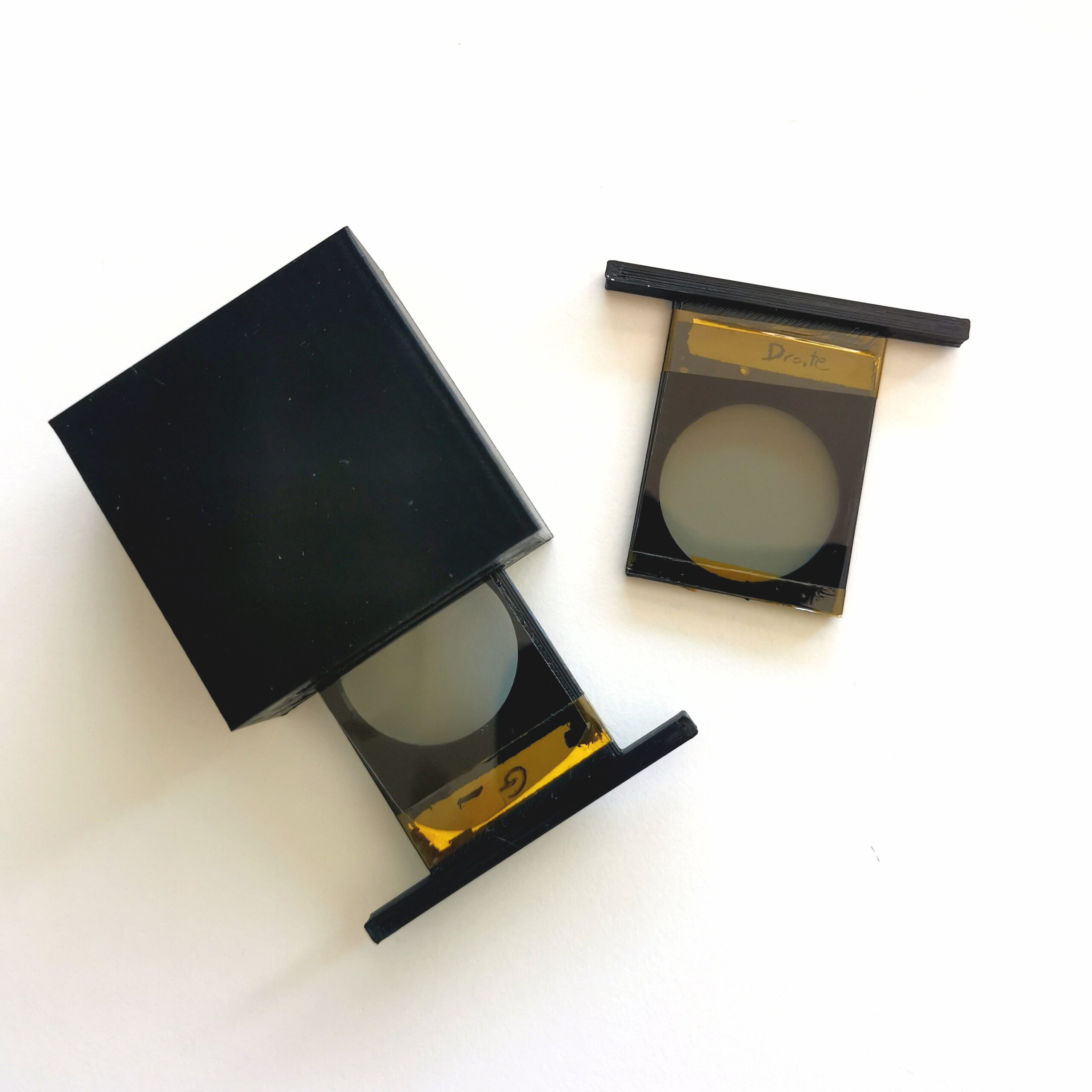
The two filters “left” and “right” of the polarimeter made with 3D cinema glasses. Each “glass” (plastic) consists of a polarising plate and a quarter-wave plate at -45° or +45° depending on the eye.
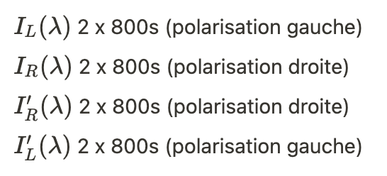
Observation strategy: The acquisitions are carried out in sequence in a precise order. Note that the exposure time (1h47 per night) is quite substantial for a target of magnitude 2.81. This is due to the “homemade” polarimeter which causes a significant loss of flux (40% less flux) and the small diameter of the instrument (SW72ED f/6 refractor).
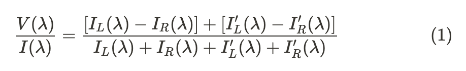
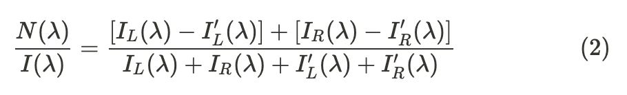
The Stokes parameters I and V corresponding respectively to the total measured intensity (strictly positive) and the circular polarisation rate, which can be positive or negative depending on the direction of rotation, are calculated using the following relationship:
The zero-polarisation spectrum for estimating the measurement error is obtained with the relation :
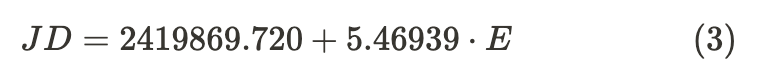
The ephemeris adopted for the phase calculation is the following (Farnsworth, G. 1932, ApJ, 75, 364):
The easiest data to obtain from the previously calculated data is the longitudinal field expressed in gauss – i.e. the component of the magnetic field in the line of sight – which is related to the Stokes parameters and through the following equation (Donati et al, MNRAS 291, 658-682, 1997):
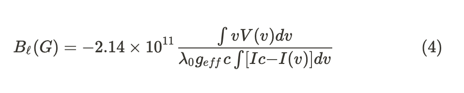
where Ic is the unpolarised continuum, v is the radial velocity, c is the speed of light in the same unit as v, λ0 is the central wavelength of the line in nm, and g is the effective Landé factor of the line.
Simulations
Here are two simulations that give a better idea of the phenomenon being measured:
Late-type active stars have structured magnetic fields at small
scale. They can be detected and characterised using high resolution spectroscopy.
resolution combined with circular polarisation analysis. The Stokes V signatures of
magnetic spots move along the profile of the line and change shape and
amplitude as a function of the orientation of the field within the spot.
Source : Oleg Kochukhov
Some early-type stars have very strong and globally organised magnetic fields. Their magnetic geometries can be described approximately with a dipole inclined to the stellar rotation axis. For such stars, we can measure and interpret the variation of the line profile in the four Stokes parameters. The Stokes V spectra provide information on the magnetic component of the line of sight while the linear polarisation spectra (Stokes Q and U) characterise the transverse magnetic field. Source : Oleg Kochukhov
Observations and treatment
The observations (eleven nights) took place between 30 June 2022 and 15 July 2022 with the equipment described below. “Observatory located in La Montagne (44) near the city of Nantes = a lot of light pollution.
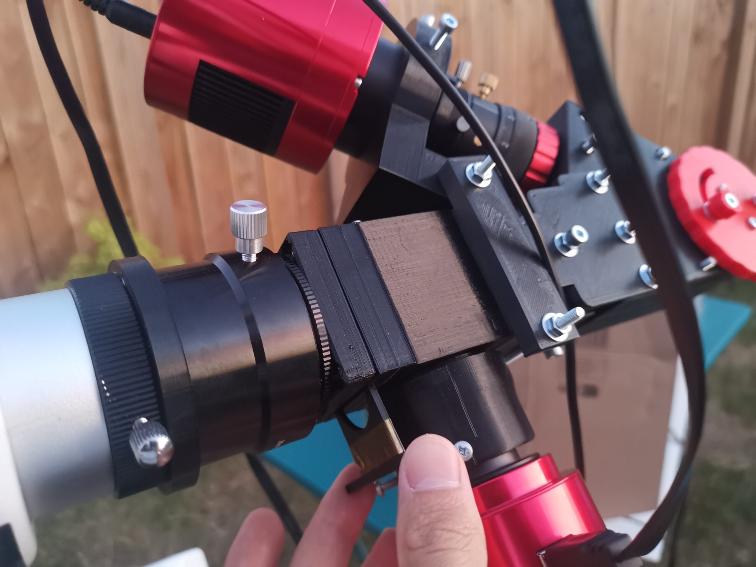
The polarimeter is placed in front of the spectro guide cube. Closer to the slot would have been better to limit the optical defects of the soft lenses of the glasses but I wished to do the simplest in term of assembly.
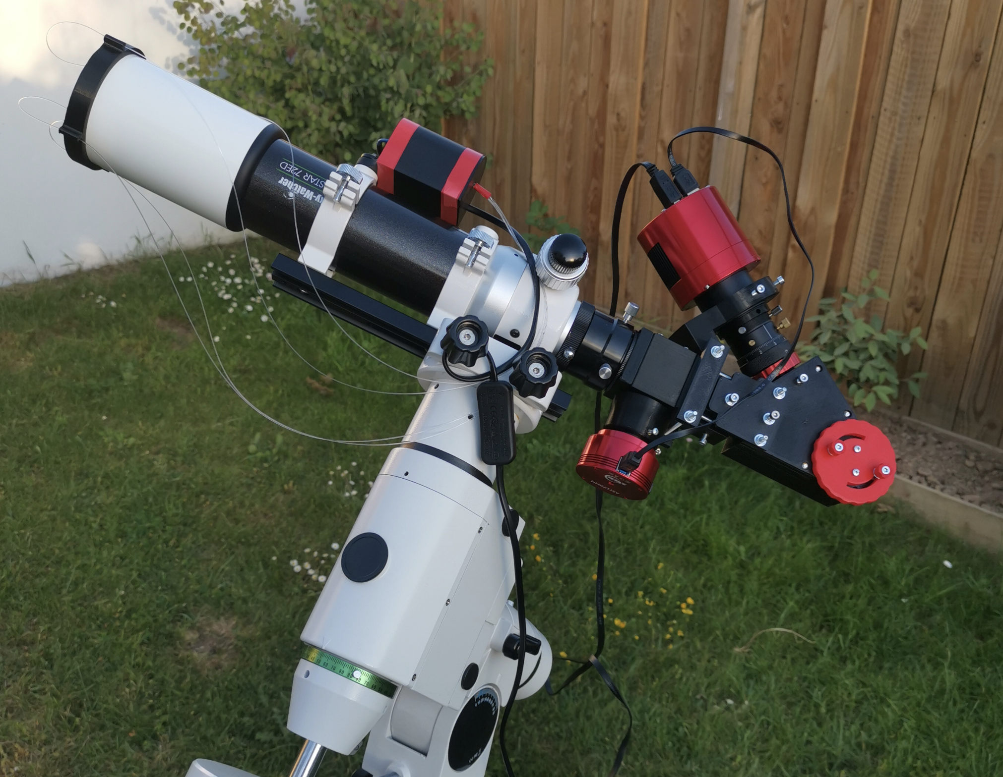
Lunette SkyWatcher 72ED f/6
Star’Ex spectrograph 2400 rpm, 80×125, 10 μm slit.
Polarimeter 3D cinema glasses (https://youtu.be/ux1rgkgdauY)
Science Camera: ASI 183 MM PRO
Guide camera: ASI 178 MM
Mount : Heq5 Pro
The spectra are acquired with SharpCap and PHD2 guidance.
The pre-processing is done with specINTI.
The calibration is carried out in lateral mode (4 optical fibres at the telescope entrance) with a neon bulb.
The average resolution of the observations with the configuration is about 25000 and the
signal to noise ratio is greater than or equal to 150.
A Python script was developed to correct the heliocentric velocity spectra, normalise the continuum, calculate the Stokes I and V parameters and present the results in graphical form.
Résults :
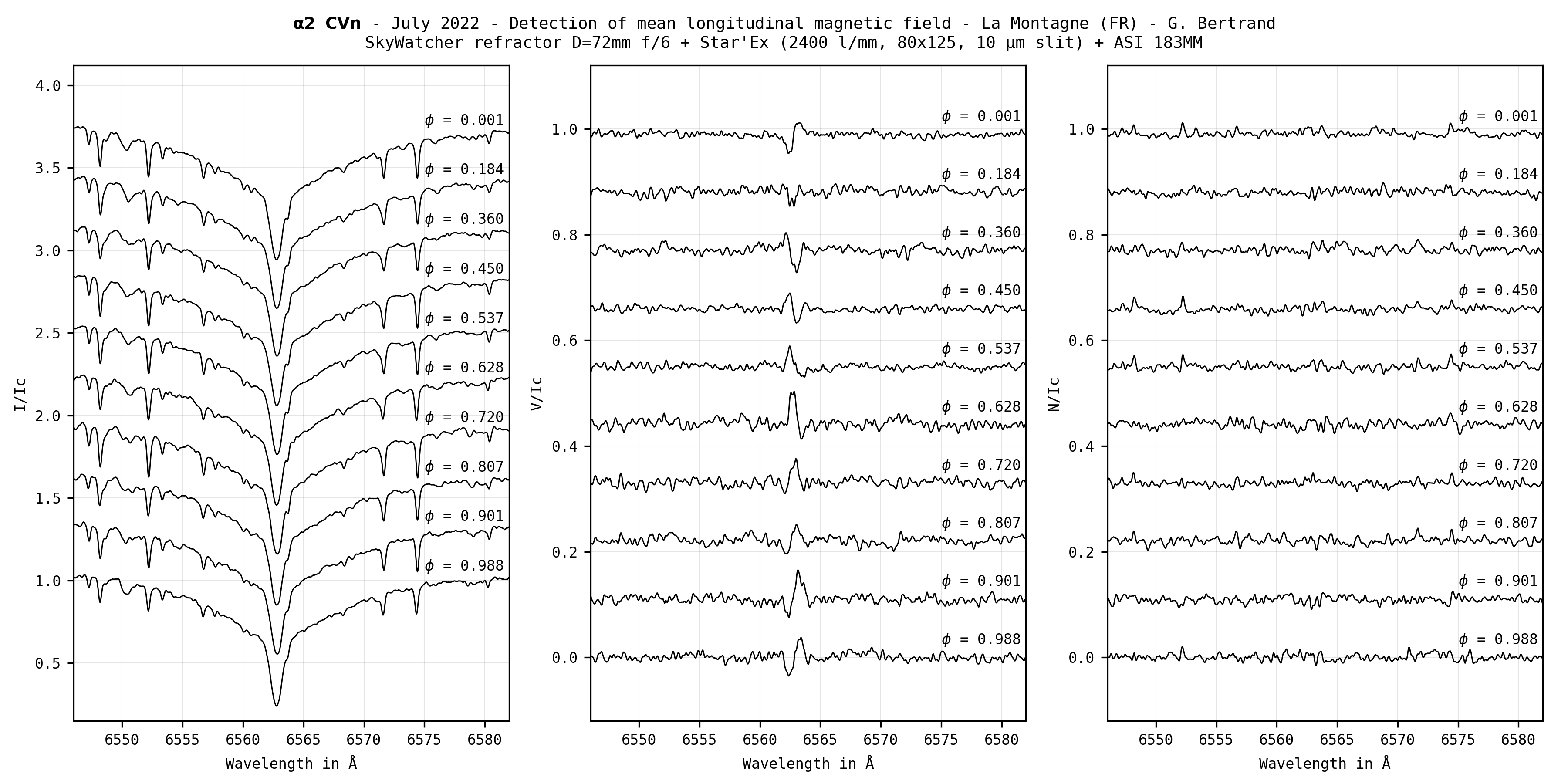
Figure 1 : From left to right
I/Ic: Total measured current
V/Ic: Circular polarisation rate
N/Ic: Zero polarisation spectrum for estimating the measurement error.
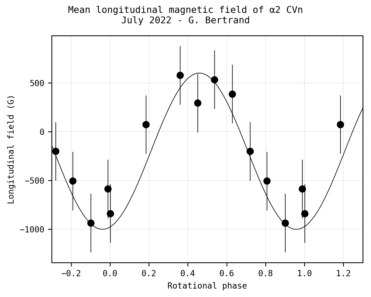
Figure 2 : Average longitudinal magnetic field calculated at the Hα line from equation (4). The error bars are calculated from the delta between the two measurement points near phase 0.
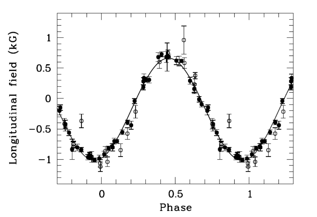
To compare with Figure 2 here are results from D. Monin et al. on the Hβ – line.
arXiv:1203.0278 (2012)
A circular polarisation signal is detected at the Hα line on the V component of the Stokes parameter (Figure 1, middle graph). The signal-to-noise ratio is not excellent but the result is supported by the zero-polarisation spectrum which does not indicate a strong measurement bias. Moreover, there is a clear correlation between these results and the results of O. Kochukhov et al. (A&A 513, A13, 2010) and C. Buil.
The polarisation rate pattern is repeated periodically as a function of phase highlighting the rotation cycle of the star (P = 5.47 days). It is from these elements that professional astronomers study the mechanisms of stellar magnetism and reconstruct maps of the magnetic field and the surface of stars. The capabilities of this small 3D printed Star’Ex spectrograph coupled with the small SW72ED scope are truly amazing! The result is beyond my expectations. It is beautiful astrophysics at the limit of instrumentation but in truth quite easily accessible with a little method.
Next step…
…reconstruct an image of the star’s surface!
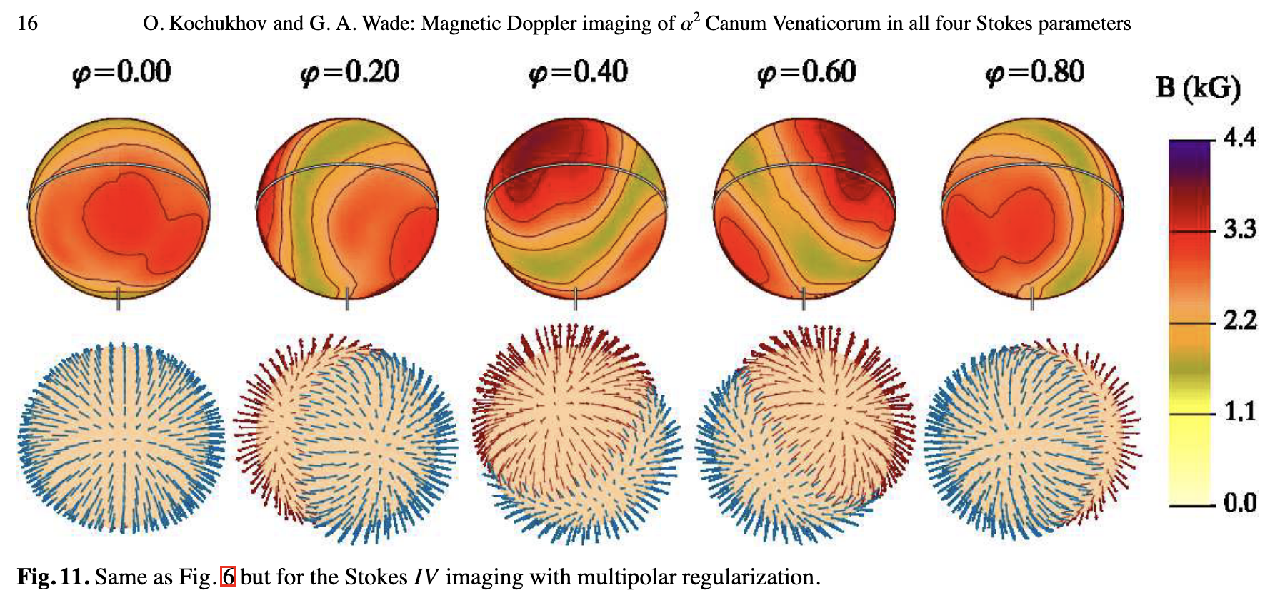
Example of the reconstruction of the Cor Caroli magnetic field using the Stokes I and V parameters. O. Kochukhov and al. 2010.
Professionals are using a complex technique to map the magnetic field and the distribution of elements on the surface of stars by inverting a high-resolution time series spectrum. This technique is called ZDI for “Zeeman Doppler Imaging”.
The periodic modulation of the Zeeman effect as a function of the star’s rotation period is used to iteratively reconstruct the magnetic field distribution on the star’s surface. Using the principle of entropy-maximising image reconstruction, this technique generates the geometry of the magnetic field (see the spherical harmonics technique) by synthesising the Stokes IV profiles to match the observations.
A prerequisite for the ZDI to work is that the width of the intrinsic line is smaller than the broadening induced by the rotation of the star (Doppler effect). This is unfortunately not the case for the Balmer lines including the Hα line. For this reason, these lines are less usable for Zeeman imaging than the lines of heavier elements (in particular Fe II 4923, 5018, 5169 Å). The latter also have a higher Landé factor than the Hα line and therefore a stronger Stokes profile signature.
However for α2 CVn stars we can model their magnetic fields by assuming oblique dipole geometries. Most modern ZDI studies find local deviations from these geometries, but at the same time confirm that oblique dipoles provide a very good first approximation to stellar magnetic fields.
After many hours of research, I managed to get my hands on a Python algorithm to do “ZDI”. It is written by C. P. Folsom (7) following the method of Donati et al (8, 12).
To date, I have developed a first Python script to prepare the spectra and create the input files that the model will consume. The model is partly constrained using the fundamental parameters of the star, the rest of the parameters are free. The idea is now to create a second script to play with these free parameters in order to converge the model to the best solution. This is the most sensitive stage… Indeed, depending on the parameters adopted, the results can differ completely.
Results to come…
Références
1. Magnetic Doppler imaging of α2 Canum Venaticorum in all four Stokes parameters
O. Kochukhov et al , A&A 513, A13 (2010)
2. Stokes IQUV Magnetic Doppler Imaging of Ap stars II: Next Generation Magnetic Doppler Imaging of α2 CVn
O. Kochukhov et al , arXiv:1402.2938v1 (2014)
3. Doppler Imaging of stellar magnetic fields III. Abundance distribution and magnetic field geometry of α2 CVn
O. Kochukhov et al , A&A 389, 420–438 (2002)
4. Measuring magnetic fields of early-type stars with FORS1 at the VLT
S. Bagnulo et al, A&A 389, 191–201 (2002)
5. Doppler Imaging of stellar magnetic fields I. Techniques
N. Piskunov and O. Kochukhov, A&A 381, 736-756 (2002)
6. Doppler Imaging of stellar magnetic fields II. Numerical experiments
O. Kochukhov et al, A&A 388, 868–888 (2002)
7. The evolution of surface magnetic fields in young solar-type stars II: the early main sequence (250-650 Myr)
C.P. Folsom et al, arXiv:1711.08636 (2017)
8. Zeeman-Doppler imaging of active stars. II. Numerical simulation and first observational results.
Donati, J. -F. et al, Astronomy and Astrophysics, Vol. 225, p. 467-478 (1989)
9. Chaîne Youtube astro-spectro
C. Buil, https://www.youtube.com/channel/UCdlVj1AAV7y_KxBIwhjChug
10. Le projet Sol’Ex & Star’Ex
C. Buil, www.astrosurf.com/solex/
11. Magnetic field structure in single late-type giants: The weak G-band giant 37 Comae from 2008 to 2011
S. Tsvetkova et al, arXiv:1612.02669v1 (2016)
12. Spectropolarimetric observations of active stars
J.-F. Donati et al, Mon. Not. R. Astron. Soc. 291, 658-682 (1997)
13. Zeeman Doppler imaging of active stars
J.F. Donati and S.F. Brown, A&A (1997)
14. Magnétométrie stellaire et Imagerie Zeeman-Doppler appliquées à la recherche d’exoplanètes par mesures vélocimétriques
Elodie E. Hebrard, https://tel.archives-ouvertes.fr/tel-01309532
15. High-precision magnetic field measurements of Ap and Bp stars
G. A. Wade et al, Mon. Not. R. Astron. Soc. 313, 851±867 (2000)