Beta Aurigae spectroscopic binary
Recommended equipment : Lhires III, eShel
Time : several observing nights

Summary
Grâce à la haute résolution du Lhires III, il est possible de séparer de nombreuses étoiles binaires spectroscopiques. Ces étoiles, qui n’apparaissent comme une seule étoile au télescope, montre un spectre dédoublé par l’effet Doppler. Nous décrivons ici dans le détail l’exemple de beta Aurigae avec des pistes pour d’autres cibles. Cet article a été originellement publié dans la revue AstroSurf et écrit en collaboration avec Pierre Noyrez pour la partie mathématique.
Introduction
Half of the stars we can watch during a night are actually binaries. While our Sun is a single star surrounded by planets (and other bodies), those binary systems are companions orbiting around their center of mass.
Visual stars can be split by looking at high power with a telescope (some require interferometric method to be visualized) while spectroscopic binaries can’t be individually seen. Their binary nature is revealed in their spectra and the radial velocity changes (Doppler-Fizeau effect) implied by their orbital movement.
Spectroscopic binaries were first discovered in 1889 at Harvard and Postdam. Dozen were soon found; Pourbaix et al. (2004) list orbits of 2386 systems in their last SB9 catalog.
In some cases, the orbit of those binaries lies in the line of sight and we can observe eclipses which are revealed by luminosity changes of the system. It was actually in 1783 when John Goodricke (1765-1787), aged 18 only at that time, did a report to the Astronomical Royal Society in London mentionning that Algol luminosity changes could come from a companion.
There are several types of eclipsing binaries among which RS CVn, z Aur, W UMa and Algols. Their variability period can be dozen of minutes to several years, epsilon Aur beeing the one with the longest period and a very interesting subject of study.
A lot of information are available from a binary system, specially for eclipsing double line spectroscopic binaries (SB2): individual masses of each star, stars radii, flux ratio, effective temperature ratio…
Beta Aurigae : a nice target… but not unique
Antonia Maury (1866-1952) has been a very active member of “Pickering’s team” working on stellar classification at Harvard observatory. She had a lot of interest for spectroscopic binaries (Hearnshaw, 1986). She discovered in 1889 the second know spectroscopic binary at that time: beta Aur.
Selection of beta Aur for this study has been decided from the SB9 catalog due to its brightness (mv=1.9) and short period (around 4 days).
Spectra have been taken between august 2006 and october 2007, all with Lhires III (Thizy 2007, 2008a and 2008b). Power of resolution l/Dl were around R=17000. Each spectrum is usually a combination of three 5min exposures. Observers are: Eric Barbotin, François Cochard, Jean-Pierre Masviel, Jose Ribeiro and Olivier Thizy.
Aurigae constellation above Saint-Véran dome (photo : Jan Karel Lameer)
Acquisition
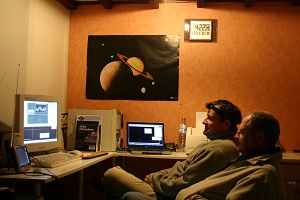
Lhires III on C14 (CALA). François Cochard & Olivier Thizy in control room… not a lot to do in autoguiding mode!
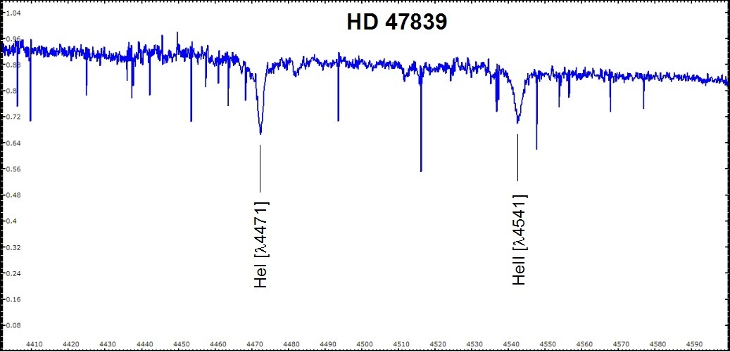
example of a spectrum with double
Halpha absorption lines (but single telluric lines)
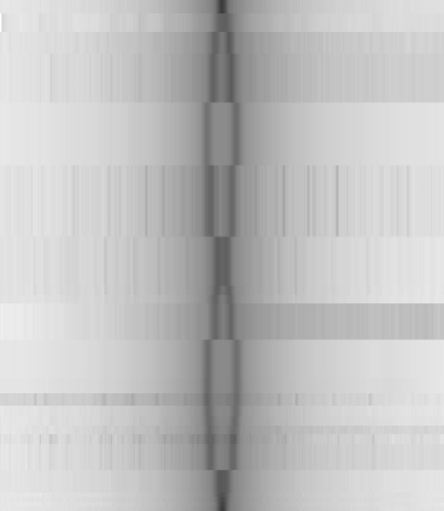
Evolution over a period, Y shift is proportional to time/phase.
The evolution of the double line over time and the shift due to Doppler-Fizeau effect. Of course, we only measure the projected speed over the line of sight, what is called v.sin(i) where ‘i’ is the inclination of the system. As the system is an eclisping binary, we can assume sin(i) close to 1.
WIRE satellite observations (Southworth, 2007) gives a period of 3.9600467300 jours. Our phase start is arbitrary set at HJD=2453827.19569.
Light curve of beta Aurigae (WIRE)
Do you like some maths ?
Each star rotates around the center of mass. We can model each orbit with the following parameters:
- a = demi grand axe,
- e = excentricité,
- P = période,
- Ω = angle de position du nœud par rapport au nord,
- ω = longitude du périastre par rapport au noeud,
- i = inclinaison du plan de l’orbite,
- T = époque de passage au périastre.
Second Keplerian law tells us that the surface speed is constant: star 2 moves faster when closer to star 1 for example. This is given by equation:
Distance ‘r’ between the two stars is given by :
Last but not least, third Kelper law tells us that total mass of the system M1+M2 (in solar masses) is linked to the semi axis ‘a’ (in astronomical unit) and period (in years) :
In a binary system, the orbital movement of a star adds a periodic radial velocity Vr to the global system RV: Vg.
First two Kepler’s laws imply that :
Time dependant component is actually n(t). In circular orbits (when masses are equal), n(t)=2.p.t/P.
Half amplitude of the RV curve (called Ki for each star) is given by :
where ‘ai’ is the semi axis of the orbit around the center of mass. Of course, K2 is seen in spectroscopic binary system where both spectra are visible. Otherwise, we can only measure K1. In beta Aur case, both K1 and K2 can be measured.
In general case where masses are different, temporal variation could be highly unsymetric as speed is faster at periastron (cf Fig below).
Measure of amplitudes provides directly the mass ratio :
In case of a single line spectroscopic binary (SB1), only the “mass function” is available and one of the mass has to be found by other means (stellar simulation for exemple) :
Mass function f(M) provides information on minimal mass of the companion.
Results on beta Aurigae
Each spectrum of b Aur have been fully processed with correction of Earth movement around the Sun (heliocentric correction). Both Ha lines have been measured with VisualSpec and with PeakFit program (minimum residuals) to compare both methods. Each measure has been transformed into speed with Doppler-Fizeau law :
where ‘c’ is the speed of light (300 000 km/s) and l0 the Ha position (l=6563.88Å).
Table 1 gives the details of each measure and Fig 7 & 8 show RV curves.
Table 1 : RV measures on b Aurigae
Radial Velocities Vs phase
SBS (Spectroscopic Binary Solver) software has been used to calculate the orbital parameters and a comparison is given on Table 2 with Nordström (1994).
Table 2 : comparison of results
Results on beta Aurigae are well aligned with Nordström except Vg ; but Popper & Carlos (1970) give Vg=-19.4 +/-1 km/s !
Other targets
There are several other targets for spectrographs such as Lhires III or eShel. Even exoplanets are now in reach with our fibre fed echelle eShel solution!
some easy targets :
- Mizar : several night project, often/always visible in northern hemisphere
- AW UMa : contact binary to do in one winter evening
- Beta Lyrae (Be star): follow up over two-three weeks
Conclusion
As shown here, motivated amateur (it does take time and observing time to run such project) can really reach out physical parameters of spectroscopic binaries. Even if the binary is well known, regular follow up can improve ephemeris calculation and orbital parameters which can vary (third companion, mass transfer…)
So… all at your high resolution spectrographs !
References :
- “Astronomie, méthode et calculs”. Agnès Acker & Carlos Jaschek. Edition Masson.
- “Double Stars”, Heintz W.D., Reidel Publishing Company (1978)
- “SB9”: The Ninth Catalogue of Spectroscopic Binary Orbits (Version September 2005). Pourbaix D., Tokovinin, A.A, Batten A.H., Fekel F.C., Hartkopf W.I., Levato H., Morell N.I., Torres G., Udry S.. Astron. Astrophys. 424, 272 (2004)
- “The realm of interacting binary stars”. J Sahade, G E McCluskey Jr, Y Kondo. Kluwer Academic Publishers (1993).
- “The analysis of stars”. J B Hearnshaw. Cambridge University Press (1986)
- “Eclipsing binaries observed with the WIRE satellite. II. Beta Aurigae and non-linear limb darkening in light curves”, Southworth J., Bruntt H., Buzasi D.L. Astron. Astrophys. 467, 1215-1226 (2007).
- “Radii and masses for beta Aurigae”, B. Nordström and K.T. Johansen, Astron. Astrophys., 291, 777-785 (1994).
- Maury A.C. 1890, Fourth report of the Draper Memorial.
- “VisualSpec”: http://astrosurf.com/vdesnoux/
- “Spectroscopy Binary Solver”, Johnson D.O., is available from: http://www.vub.ac.be/STER/JAD/JAD10/jad10_3/jad10_3.htm
- A local copy of Spectroscopy Binary Solver is also available.
- Logiciel “Mathematica”, http://www.wolfram.com/
- Logiciel “PeakFit”, http://www.systat.com/
- Applet Java, Terry Herter, http://instruct1.cit.cornell.edu/courses/astro101/java/binary/binary.htm
- Applet Java, J. Köppen, http://astro.u-strasbg.fr/~koppen/jeanlouis/BinaryStar.html
ANNEXE – OVERALL SHAPE OF RADIAL VELOCITY
It is interesting to remind that radial velocity Vr over time is not as obvious as it look like in this particular exemple where the orbits are almost circular. Here are the four steps to go through
1) mean anomaly M(t) :
2) excentric anomaly E(t) by resolving kepler equation :
This equation can’t be resolved but solution is unique and numerical methods have been developped to solve it.
3) true anomaly n(t) by resolving equation :
4) finally Vr(t) with equation :
Below are some exemple ((K = 110 km.s-1 ; = -20 km.s-1) calculated by Pierre Noyrez using previous equations and numerical from Mathematica® 6.
Radial Velocity curves for several values of e & ω
One can see that the overall shape gives some information on the orbital parameters. Comparing theoritical and actual curves can provide a first estimate of e & o parameters.