How to choose your autoguiding camera in 2020 ?

By Olivier Garde & François Cochard

In astronomical spectroscopy, guiding camera is an important element, since it’s what makes it possible to point the right target (star, nebula, etc.), then to ensure precise guiding to inject the maximum light into the spectrograph slit. We must never forget that what differentiates a “beautiful” observation from a bad observation is only the amount of light injected into the spectroscope!

The range of guiding cameras is constantly evolving, and the CCD cameras that we recommended a few months ago (Atik Titan and 314L +) are no longer available today. The cameras that are within our reach are now all in CMOS technology; this change in technology gives us the opportunity to look in detail at the selection criteria for such a camera.

At first glance, CMOS technology completely replaces the CCD, with no apparent effect on the user. In fact, there are still notable differences:

1.The price of CMOS sensors is significantly cheaper than CCDs.

2. CMOS camera pixels are generally smaller.

3. The reading dynamic is lower (for the moment) in CMOS (12 bits in CMOS instead of 16 bits in CCD in most cases).

4. The thermal signal, which had almost disappeared with the latest CCDs, reappears on CMOS, which requires effective cooling to keep the same level of performance.

5. We also see on CMOS sensors a phenomenon called “Amp glow”, linked to thermal sensitivity. This results in bright areas in the image. This effect is more or less corrected according to the manufacturers.

6. The inherent defects in the sensors are different: we no longer have hot CCD pixels, but we see “telegraph noise” appear, which can give an outlier to a given pixel in a given image. The hot pixels of the CCDs always remained in the same place, while the deviant pixels in CMOS move from one image to another (it is no longer an internal defect in the pixel, but a defect in the pixel read time).

7. Reading noise from CMOS is significantly lower than from CCD.

8. However, it’s no longer possible to do “analog binning”. In CCD, you could gather several pixels to improve the sensitivity (at the cost of a loss of resolution), this is no longer possible in CMOS (where each pixel has its own reading system). One can of course always do a digital binning (after analog reading of the pixel), but then one no longer takes advantage of the fact of carrying out only one reading for a group of pixels (4, 9, 16, etc…)

With these technical elements, it seems appropriate to look at the current offer (January 2020) of guiding cameras, for its application to astronomical spectroscopy.

Depending on your equipment and your project (educational, scientific …), and the type of target you want to observe, the choice may be different. This article will list the various criteria to take into account to determine the best camera to guarantee a good autoguiding and quality pointing in spectroscopy. It is based on the cameras existing at the time of publication of this article.

Quantum efficiency

One of the first criteria to take into account is the quantum efficiency of the sensor. However, to date, most of the latest cameras on the market have a maximum quantum efficiency of around 74 to 77%, the peak of which is around 500 to 550 nm. It will therefore not be discriminating in practice.

Pixel size

The cameras have different pixels sizes varying by a factor of around 4 (2.1 µm for the smallest pixels, up to 9 µm for the largest). The size of the pixel has several effects:

• Larger a pixel is, more sensitive it is and therefore can detect weaker targets with the same exposure time. It’s therefore important to take this criterion into account according to the magnitude of the targets that we intend to point.

• But on the other hand, we must take care to always keep a correct sampling, to say that the pixel must be smaller than the smallest detail given by the guide optics. In spectroscopy, it’s essentially the star image size on the guidance sensor that must be considered. This size depends mainly on the quality of the sky (seeing), and the focal length of the instrument (possibly corrected for the reduction in focal length of the guiding element).

With a small focal length instrument (say less than one meter focal length), it’s better to check this point with this simple equation :

with :
E = setup sampling (optics + camera) in arcsecond / pixel
P = pixel size in µm
F = optical focal length in mm

According to the Nyquist-Shannon criteria, it’s necessary to sample the signal (here the image of the star) with a factor x2 or even x3. In any case, it is better to oversample than to undersample.

In practice, you should always prefer large pixels, except to use an instrument with a short focal length (<1m) or be in a site with an exceptional sky (very good seeing). In these cases, a quick sampling calculation is welcome.

The sensor field

The field of the autoguiding sensor must be large enough to identify the target, either visually (by comparing for example the stars of the field with a star map) or automatically (by a recognition of the field via astrometry.net for example ). If the field is too small, it will not have many stars and it will be difficult to identify certainty the target.

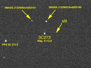
Example of a field with a 1/3′ sensor (4,83 x 3,6mm)
(Image : Olivier Garde)

The image above shows the field of a 1/3 inch sensor used on a C14 + focal reducer bringing the native focal length of the telescope to about 2.5 m. The target is the quasar 3C 273 with a magnitude V = 12.9, the unit exposure time to obtain this image is 3s in 1×1 binning (pixel of 7.4µm). We see that there are not many stars visible in the sensor field. Field recognition can be tricky, especially if the pointing of the telescope is not precise (in this case the target will not even be visible on the sensor).

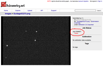
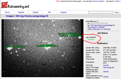
Result of field identification with astrometry.net

If you upload this image from the astrometry.net website, it’s not able to recognize the field. In the case of this setup (C14 @ f / d7), it would be beneficial to use a larger sensor, for example a Sony IMX174 sensor whose surface is more than 2x larger than a 1/3 ‘inch sensor.

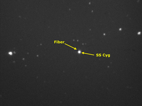
Autoguiding field with a RC400 @ f/d 6,3 and a Sony ICX-285AL sensor
(image : Olivier Garde)

The image above shows SS Cyg star (mag. V = 7.70) on a 9 x 6.7mm sensor. There are many more stars visible in the field (area of ​ Cygnus constellation which is quite dense in star). In this case, it is easy to identify the target.

By uploading the image to astrometry.net, there the identification of the field is successful.

Depending on the focal length of your instrument, you must therefore choose a sensor large enough to be able to identify the target with certainty

In some cases, when the target is particularly weak, it may be necessary to guide on a star close to the target. In this case, the guide star will be outside the slit. A large sensor then gives more chances to find a bright star in the field.

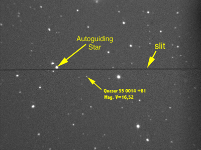
Autoguiding field of Quasar S5 0014 +81 (9 x 6,7mm sensor)
(Image : Olivier Garde)

Here the target is a quasar of magnitude V = 16.5, we cannot guide on the target directly because too weak and invisible for exposure times of a few seconds, it is therefore necessary to have a brighter star in the sensor field  on which the autoguiding will be carried out.

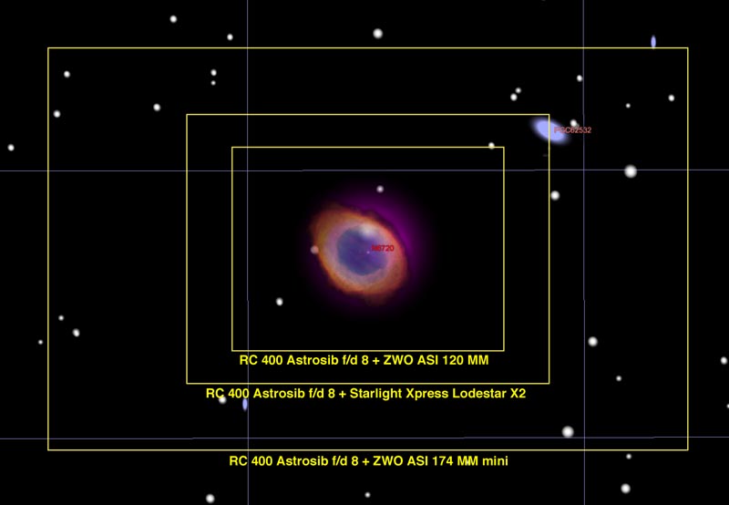
The image above shows 3 fields of different sensors generally used in autoguiding. The smallest is the field obtained with sensors like the ATIK Titan, ASI 120MM, QHY 5LII or SBIG STI. The largest corresponds to cameras equiped with SONY IMX 174 sensors.

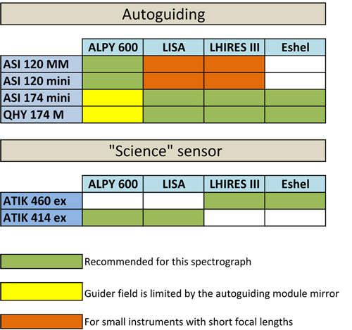
Caution : in some spectroscopes, the guiding mirror – which returns the image from the telescope to the guiding sensor – limits the effective guiding field. This is particularly the case for the Alpy 600 guidance module; in this case, it is not useful to have a very large sensor.

ST4 guiding interface

The ST4 guiding interface allows you to control the mount through the camera, by simulating pressing the displacement keys of the mount. Most autoguiding software has this functionality. The alternative solution is to control the mount by a dedicated computer protocol, specific to each mount. If there is a choice between mount control with ascom driver of the mount with ST4 autoguiding interface, this latter solution should rather be preferred for 2 reasons:

• Guiding is more responsive and precise via the ST4 port (especially visible on large focal lengths, old PCs with old OS like XP or W7)

• Some mounts don’t allow self-guiding via the mount driver using an ASCOM interface, very widespread today, and very practical. This concerns certain professional observatory or custom mount.

Having an ST4 interface is therefore not strictly necessary, but provides a guarantee of precise guiding.

Cooling

Cooling a camera allows long exposure times, while containing the thermal signal (and its associated noise) at acceptable levels. In most cases, the guiding exposure times are short (a few seconds at most), and cooling is therefore unnecessary. But if you plan to observe weak targets, then cooling becomes necessary – especially with a CMOS sensor.

A long exposure time also makes it easier to identify the target and make automatic field recognition.

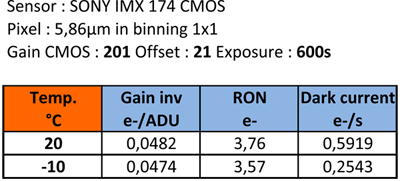
The table above shows the thermal signal noise decrease as a function of the sensor cooling over a long time exposure of 600s. In some cases (for very weak targets), it may be necessary in spectroscopy to place 1 to 2 minutes on the autoguiding sensor to properly identify the target and its positioning on the spectrograph slit. In this case the use of a cooled camera is a valuable asset.

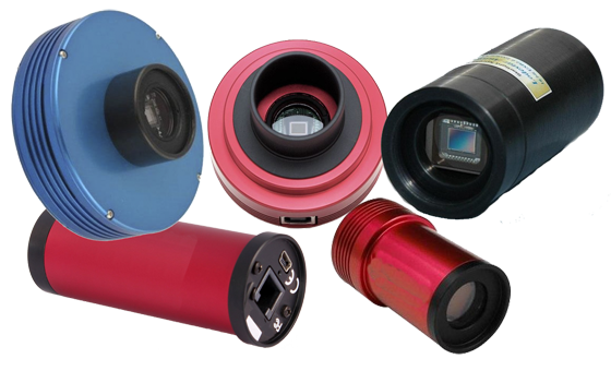
Which camera to choose ?

There are many autoguiding cameras available on the market and it is not always easy to find the model corresponding to its instrumentation and the budget that we have set. Here’s a table showing some autoguiding cameras, some are no longer sold (ATIK 314L + or ATIK Titan) but many amateur astronomers have one. They can also still be purchased in second-hand.

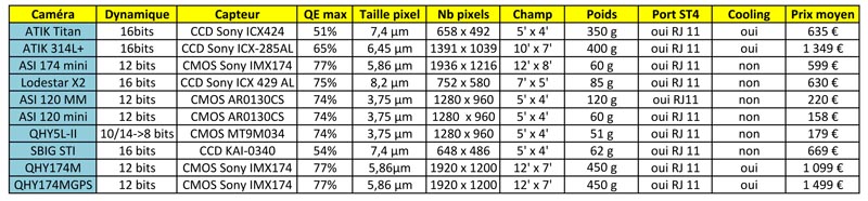
• All the sensors are monochrome
• The indicated field is for a 400mm telescope @ f / d 8 -> 3200 mm focal length

Our camera recommendations

Here is a table showing our recommendations for autoguiding cameras for use in spectroscopy on models currently on the market (January 2020)