The Whoppshel in action on a 60 cm telescope
By Olivier Garde

The Hubert Reeves observatory in Mars (Ardèche – south of France)
(Copyright photo : Olivier Garde)
The Whoppshel spectrograph has been designed for telescopes of 0.6 to 1m in diameter class (or even beyond). The resolution R = 30000 of this instrument indeed requires a significant diameter to collect enough light.
Several times we have received the question of the accessible limit magnitude with this spectroscope on a 60cm telescope; in order not to make a purely theoretical answer, we had to make a full-scale test on a telescope of this diameter.
We had the opportunity to use for a few weeks the first Whoppshel copy on the RC600 telescope of the Hubert Reeves observatory in Mars (Ardèche – south of France).
We would like to thank the community of town Valeyrieux, owner of the telescope as well as the Mars Astronomy Club (CAM) and its president Daniel Verilhac who warmly welcomed us, assisted for installation and made observations on this great instrument.
The Hubert Reeves Observatory
Located in a small village : Mars in Ardèche (south of France) at 1 030 m above sea level, the observatory benefits a 360-degree clear horizon and a sky of great quality.A 4.50m dome houses an Italian-made Officina Stellare telescope: a Ritchey-Chretien optic, 600mm diameter open at F / 8. It is mounted on a German equatorial mount direct drive Nova 200 built by the French company Alcor System.
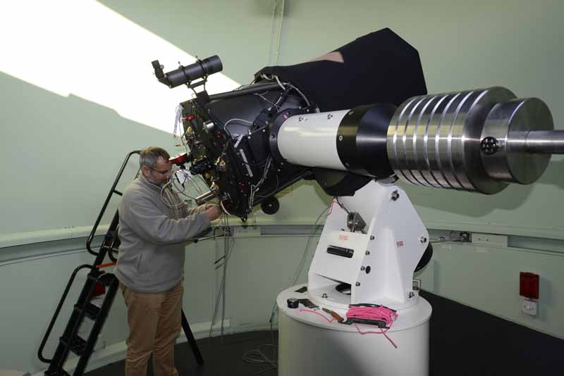
The RC600 on its mount Nova 200
(Copyright photo : Olivier Garde)
To inject the light collected by the telescope onto the 50μm optical fiber, we use an injection unit from Shelyak Instruments at F/6. With the telescope open at F / 8, we use an Astro-Physics CCDT67 (x 0.67) focal length reducer to reduce the focal length of the telescope to F / 5.4. Note that Shelyak Instrument can now offer injection unit with multiple openings, incorporating an internal focal length reducer. It is thus possible to have unit at F / 6, F / 7, F / 7.8 and F / 9.
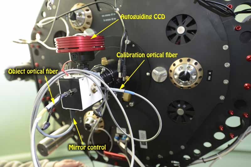
The injection unit mounted on the RC600
(Copyright photo : Olivier Garde)
The injection unit is mounted with its focal reducer, on the eyepiece holder of the RC600 (2 inches). It allows to perform several tasks:
-
injection of the light flux into the optical fiber “Object” connected to the spectrograph.
-
Autoguiding on the target
-
Realization of calibration images (Flat, spectral lamp, LED)
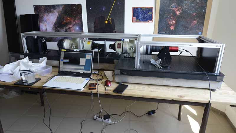
Whoppshel assembly
The whoppshel is an echelle spectrograph mounted on an optical bench of 2.10m long and 0.6m wide. The total mass is about 80 kg.
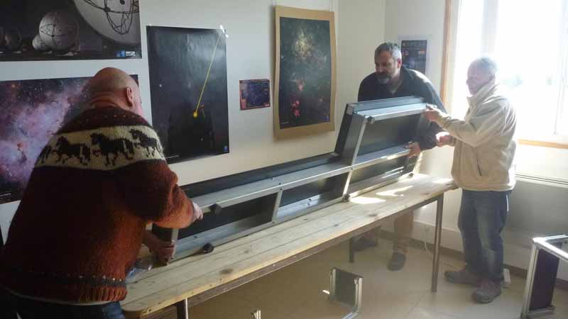
Assembly of the 2 optical benches
(Copyright photo : Daniel Verilhac)
The whoppshel being assembled
(Copyright photo : Olivier Garde)
The various preassembled modules of the spectrograph are fixed on the optical bench: the optical fiber injection support, the 90-degree deflection mirror, the two optics Takahashi FSQ-106, the grating module, the cross-disperser (3 prisms) and the CCD camera with its lens. The detailed constitution of this instrument was described in this article.
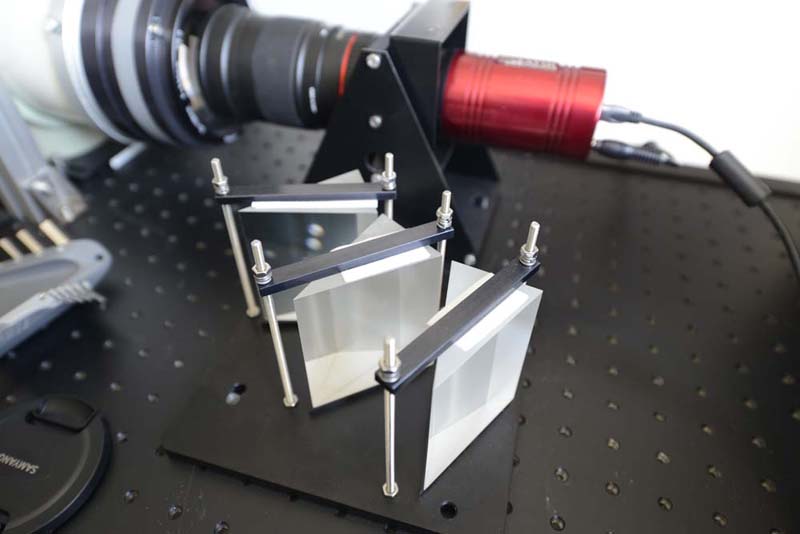
The cross-disperser module and the CCD camera
(Crédit photo : Daniel Verilhac)
The cross-disperser module, which separates the different orders, consists of 3 prisms custom designer. They are arranged in a precise manner on a support which is fixed on the optical bench of the spectrograph at the output of the second refractor FSQ-106. The CCD camera is equipped with a 135mm optics open at F / 2.

The Whoppshel once assembled
(Copyright photo : Olivier Garde)
A black metal cowling covers the entire spectrograph to protect it from stray lights and dust. The assembly is very stable mechanically, but it is preferable that the storage room is also stable in temperature during the acquisition of the spectra if one wishes to measure precise radial velocities.
The results
We tested the spectrograph for several nights thanks to the regular presence of Daniel Verilhac at the observatory. He was able to produce dozens of spectra of stars despite a weather not always favorable. Often it would have been useful to ask longer on some targets to improve the signal-to-noise ratio of the spectrum, but the passage of clouds during the observation periods prevented us from doing so. A short overview of the observations made on various stars with various astrophysical interests …
HD 123299
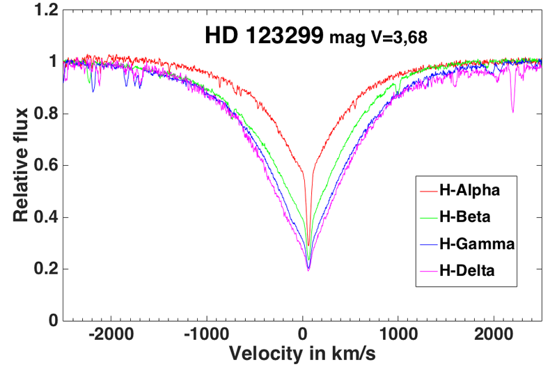
The first target was the star HD 123299 (Alpha Dra) of magnitude V = 3.68. It allowed us to calculate the instrumental response of the spectrograph by comparing its spectral profile with a theoretical spectrum of the Pickles database. It is a AOIII type profile and we realized 5 exposures of 600s with an ATIK 460ex CCD camera in binning 1×1 and cooled to -1 ° C (the ambient temperature of the room did not allow us to cool more) .
The graph below shows the corrected spectrum of the instrumental response calculated from this star (Alpha Dra). In blue, the curve obtained with the Whoppshel, in red, the curve of the Pickles database of a A0III type star.
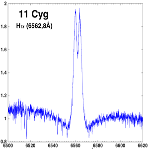
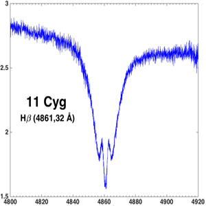
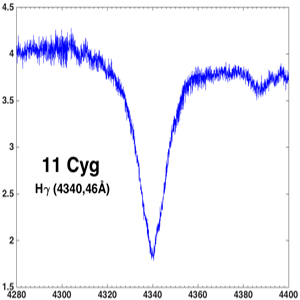
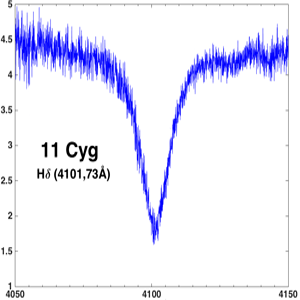
11 Cyg
Here is the spectrum of 11 Cyg, a Be star of magnitude V = 6,03. Here we made 5 exposures of 900s, some with cloud passages. The graphs below show the profile of hydrogen lines from H Alpha (6562.8 Å) to H Epsilon (3970.07 Å).
11 Cyg
H Alpha (6562,8 Å)
11 Cyg
H Beta (4861,32 Å)
11 Cyg
H Gamma (4340,46 Å)
11 Cyg
H Delta (4101,73 Å)
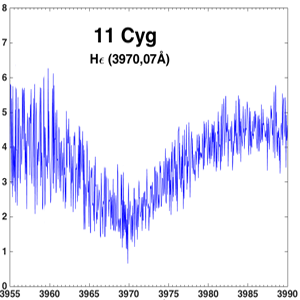
11 Cyg
H Epsilon (3970,07 Å)
Chi Dra
Another “fashionable” observation subject: chromospheric stars. This is to see any emissions in H & K Calcium lines (CAII). This spectrum of Chi Dra (mag V = 3.58) shows that the Whoppshel is able to go so far into the near UV.
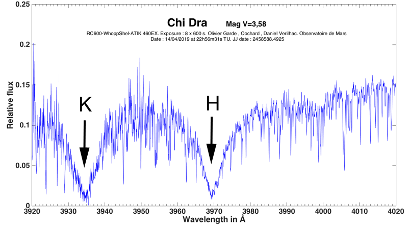
Chi Dra spectrum (mag V = 3.58) centered on the H and K Calcium II lines, respectively at 3968.47 Å and 3933.66 Å.
8 exposures of 600s (ATIK 460ex in 1×1 binning)
WR 140
The Wolf-Rayet stars (WR) show broad emission lines, clearly visible in this spectrum of WR140, of magnitude V = 6.85. 3 exposures of 1200s, exactly one hour total exposure. And when we “zoom” in each strip, what details can be observed!
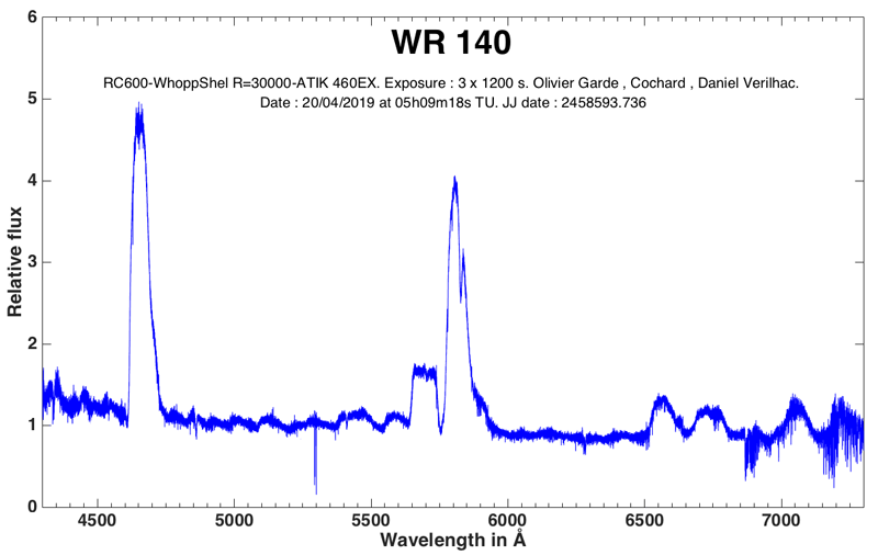
WR 140 spectrum
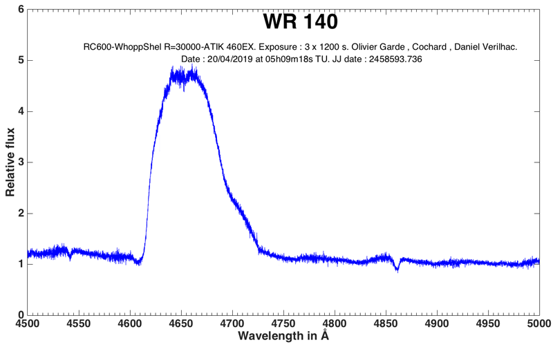
Details of WR 140 spectrum (between 4500 and 5000 Å)
HD 191378
The limiting magnitude accessible with this instrument depends, of course, on the total exposure time and the desired Signal / Noise Ratio (SNR). We limited ourselves during this campaign to a duration of observations around one hour. The faintest star we observed is HD 191378, a Be star of magnitude V = 8.99 with only 4 exposures of 1200s (1h20 total exposure). We see that the spectrum is noisy in the blue … but still: magnitude 9 with a resolution of R = 30,000!
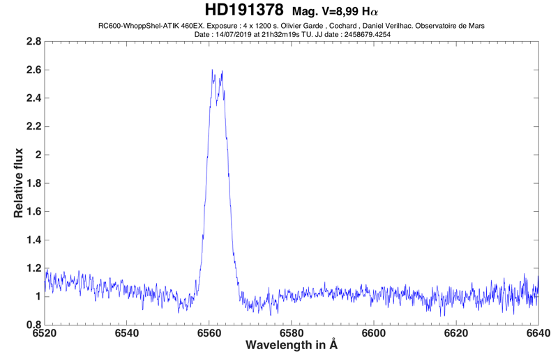
HD 191378 H Alpha
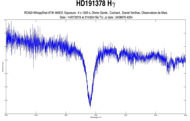
HD 191378 H Gamma
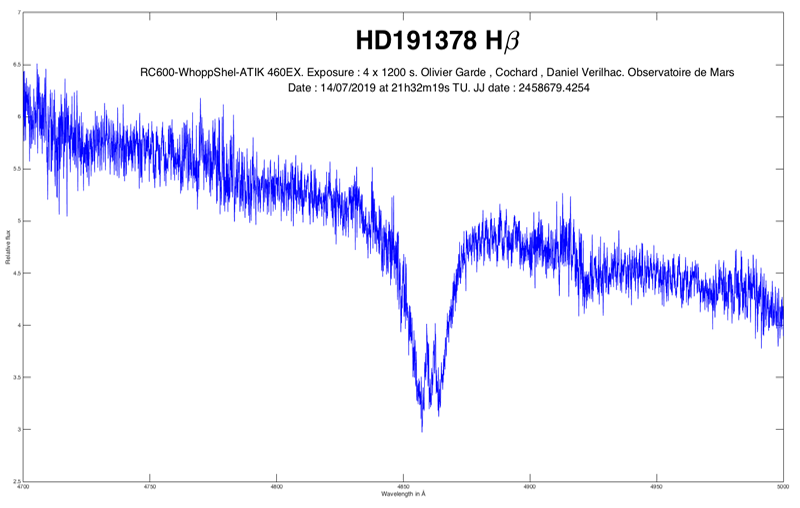
HD 191378 H Beta
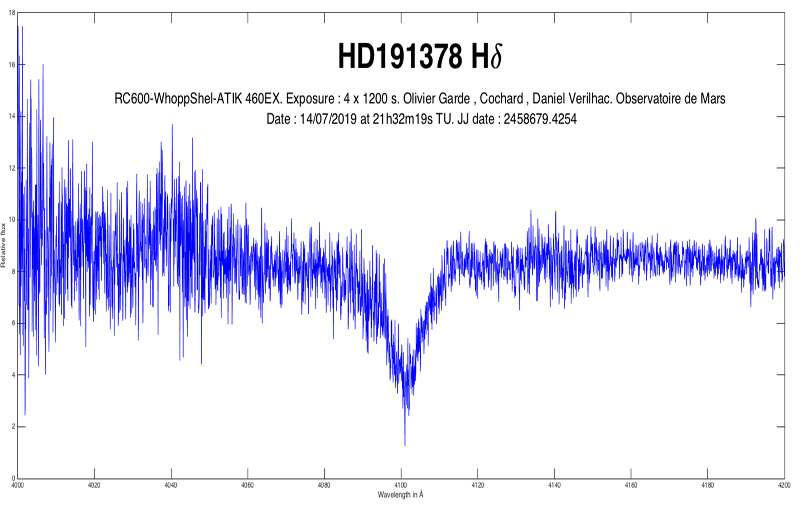
HD 191378 H Delta
Many other spectra have been produced, including several spectra of Be stars that you can download from the Bess spectral database.(select the RC600-WhoppShel-ATIK 460EX instrument).
Some key numbers
Here is the calculation result provided by ISIS (version 5.9.3) for each order on the 11 Cyg spectrum. Order 47 is the first order in red, and order 86 is the last in blue. The calibration RMS is excellent with average values of the order of 0.003 Å.
Ordre #47 : RMS = .0611 – Nb. raies = 9 FWHM = 8.09 – Dispersion = .062 A/pixel – R = 14420.5
Ordre #48 : RMS = .0677 – Nb. raies = 7 FWHM = 9.28 – Dispersion = .061 A/pixel – R = 12516.9
Ordre #49 : RMS = .0015 – Nb. raies = 8 FWHM = 7.38 – Dispersion = .061 A/pixel – R = 15567.5
Ordre #50 : RMS = .0073 – Nb. raies = 8 FWHM = 6.41 – Dispersion = .059 A/pixel – R = 18013.3
Ordre #51 : RMS = .0032 – Nb. raies = 11 FWHM = 5.69 – Dispersion = .058 A/pixel – R = 20194.3
Ordre #52 : RMS = .0032 – Nb. raies = 11 FWHM = 5.20 – Dispersion = .057 A/pixel – R = 22349.0
Ordre #53 : RMS = .0042 – Nb. raies = 12 FWHM = 4.59 – Dispersion = .057 A/pixel – R = 24868.4
Ordre #54 : RMS = .0017 – Nb. raies = 10 FWHM = 4.23 – Dispersion = .055 A/pixel – R = 27028.2
Ordre #55 : RMS = .0021 – Nb. raies = 15 FWHM = 4.01 – Dispersion = .054 A/pixel – R = 28723.9
Ordre #56 : RMS = .0007 – Nb. raies = 10 FWHM = 3.91 – Dispersion = .053 A/pixel – R = 29480.5
Ordre #57 : RMS = .0018 – Nb. raies = 13 FWHM = 3.86 – Dispersion = .052 A/pixel – R = 29763.2
Ordre #58 : RMS = .0024 – Nb. raies = 12 FWHM = 3.85 – Dispersion = .051 A/pixel – R = 29776.6
Ordre #59 : RMS = .0025 – Nb. raies = 12 FWHM = 3.85 – Dispersion = .051 A/pixel – R = 29763.7
Ordre #60 : RMS = .0016 – Nb. raies = 12 FWHM = 3.94 – Dispersion = .049 A/pixel – R = 29543.1
Ordre #61 : RMS = .0020 – Nb. raies = 14 FWHM = 3.93 – Dispersion = .049 A/pixel – R = 29312.2
Ordre #62 : RMS = .0029 – Nb. raies = 13 FWHM = 3.94 – Dispersion = .048 A/pixel – R = 29158.7
Ordre #63 : RMS = .0072 – Nb. raies = 16 FWHM = 4.19 – Dispersion = .047 A/pixel – R = 27528.6
Ordre #64 : RMS = .0054 – Nb. raies = 11 FWHM = 4.17 – Dispersion = .046 A/pixel – R = 27744.9
Ordre #65 : RMS = .0045 – Nb. raies = 12 FWHM = 4.23 – Dispersion = .046 A/pixel – R = 27077.1
Ordre #66 : RMS = .0029 – Nb. raies = 14 FWHM = 4.36 – Dispersion = .045 A/pixel – R = 26441.2
Ordre #67 : RMS = .0034 – Nb. raies = 13 FWHM = 4.38 – Dispersion = .044 A/pixel – R = 26347.2
Ordre #68 : RMS = .0218 – Nb. raies = 13 FWHM = 3.82 – Dispersion = .044 A/pixel – R = 29917.4
Ordre #69 : RMS = .0006 – Nb. raies = 8 FWHM = 4.47 – Dispersion = .043 A/pixel – R = 25935.4
Ordre #70 : RMS = .0018 – Nb. raies = 9 FWHM = 4.40 – Dispersion = .043 A/pixel – R = 25955.4
Ordre #71 : RMS = .0026 – Nb. raies = 10 FWHM = 4.26 – Dispersion = .042 A/pixel – R = 26941.9
Ordre #72 : RMS = .0007 – Nb. raies = 11 FWHM = 4.18 – Dispersion = .042 A/pixel – R = 27238.5
Ordre #73 : RMS = .0018 – Nb. raies = 12 FWHM = 4.23 – Dispersion = .040 A/pixel – R = 27543.4
Ordre #74 : RMS = .0055 – Nb. raies = 10 FWHM = 4.39 – Dispersion = .040 A/pixel – R = 26419.2
Ordre #75 : RMS = .0016 – Nb. raies = 11 FWHM = 4.18 – Dispersion = .039 A/pixel – R = 27715.6
Ordre #76 : RMS = .0011 – Nb. raies = 9 FWHM = 3.83 – Dispersion = .039 A/pixel – R = 29945.7
Ordre #77 : RMS = .0012 – Nb. raies = 10 FWHM = 4.01 – Dispersion = .038 A/pixel – R = 28923.0
Ordre #78 : RMS = .0021 – Nb. raies = 13 FWHM = 4.06 – Dispersion = .038 A/pixel – R = 28466.2
Ordre #79 : RMS = .0024 – Nb. raies = 12 FWHM = 4.27 – Dispersion = .037 A/pixel – R = 27137.1
Ordre #80 : RMS = .0034 – Nb. raies = 11 FWHM = 3.84 – Dispersion = .037 A/pixel – R = 29738.4
Ordre #81 : RMS = .0018 – Nb. raies = 11 FWHM = 3.73 – Dispersion = .036 A/pixel – R = 31107.6
Ordre #82 : RMS = .0036 – Nb. raies = 9 FWHM = 4.07 – Dispersion = .035 A/pixel – R = 29097.0
Ordre #83 : RMS = .0210 – Nb. raies = 9 FWHM = 3.51 – Dispersion = .036 A/pixel – R = 32916.2
Ordre #84 : RMS = .0958 – Nb. raies = 10 FWHM = 3.34 – Dispersion = .035 A/pixel – R = 34570.3
Ordre #85 : RMS = .0317 – Nb. raies = 10 FWHM = 3.02 – Dispersion = .035 A/pixel – R = 37907.5
Ordre #86 : RMS = .1350 – Nb. raies = 11 FWHM = 3.43 – Dispersion = .034 A/pixel – R = 33108.4
Conclusion
This observation campaign conducted in a beautiful observatory, on a high quality instrument, but with a rather ungrateful weather allowed us to confirm the performance of Whoppshel in real conditions – with exposure times around of one hour :
- a 60 cm telescope provides resolution spectra of around 30,000 from 3900 Å to 7600 Å.
- Without being in optimal weather conditions and with an object fiber of 50 microns, objects can be observed up to magnitude 9.
- The potential of this same instrument with a fiber of 105 microns – of course with a lower resolution of 15,000 – is vast.
At the time of writing, we have just learned that the Nobel Prize in Physics 2019 was awarded (among others) to two Swiss researchers, Michel Mayor and Didier Queloz, for their discovery of the first exoplanet 51 peg b. This discovery was made in 1995 at the Haute Provence observatory, where we organize a Spectro Star Party every year. It is a great emotion for us: they are people who are models for us, it’s a place and a familiar instrument, and by devoting ourselves to astronomical spectroscopy, we work as a result of these researchers to better to understand the Universe around us
And you know what ? The Whoppshel is a wonderful tool to explore the world of exoplanets!