Measure star temperature

Recommended equipment : Lhires III, eShel, Lisa, Alpy, Star Analyser
Time : 4h

French philosopher Auguste Compte (1798-1857) became very famous when he wrote in 1835 about stars: “… we will never know, by any mean, chemical composition of the astronomical bodies, their mineralogy or the nature of the organized bodies living on their surface, etc.”. His 19th positive philosophy course is now sadly famous !

Auguste Comte shouldn’t be aware about Joseph Fraunhofer (1787-1826) work who studied in 1814 solar spectrum and discovered multiple absorption lines. Later, Bunsen and Kirchhoff made tremendous step with their chemical composition studies based on spectroscopy. In this article, we will focus on how modest amateur backyard tools can measure the star temperature by studying overall spectrum profile.

Beginning of XXème century, physician Max Planck (1855-1947) gave a mathematical formula of the energy distribution emitted by a black body. From this work, Albert Einstein (1879-1955) explained in 1905 the photovoltaic effect and conluded light was made by discrete particles – photons. Since then, the double identity of light (wave and particle) drove numerous experiments. A photon is an electrical nutral particile, without mass, traveling in straight line whose energy is inverse proportional to its wavelength l: E = hc/l with h Planck constant (6.62.10-34 J.s) and c the speed of light in empty space (299792 km.s-1).

This photon particule theory opened the door to Sir Arthur Schuster (1851-1934) & M. Schwarzschild (1873-1916) on stellar atmosphere theories and allowed the first quantitative estimates on stellar effective temperature by german astronomers from Postdam J. Wilsing (1856-1943) & J. Scheiner (1858-1914).

Temperature is defined as a particule movement. Hot air is characterized by particles beeing more agitated than in cold air. For a star, effective temperature is defining the particule agitation, whose visible sign is the radiation (light) emitted by the star.

Stellar radiation we see comes from external layers of the star called photosphere. Its thickness is very small compared to the star size overall, like an apple skin. Internal photon take million years to travel through not because of star size but because of the internal extremely high temperature and photons are quickly absorbed then reemitted in another direction to finally escape the star from the photosphere.

After it escape, photon lives a peaceful life traveling in straight direction with very small chance to hit an object (dust for exemple) before hitting your telescope mirror and precious spectrograph !

Planck’s law

In first approximation, radiation emitted by a star is similar to a black body one. I always find strange to compare a bright star with a black body, but this is the same as the cooking plate wich becomes red as it get hotter. If the temperature were increasing higher, it would become blue! But without energy, the cooking plate is black. Its color depends on its sole temperature.

Stars are the same. A star with a null temperature would not shine and would reflect no light back. Theorist considere stars as a black box where nothing enters in and light shining out depends only on the agitation of particles inside.

Interesting property of black body radiation is that the temperature T [°K] and intensity at wavelength l [m] is given by Planck’s law :

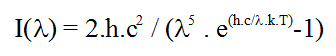
with k the Boltzmann constant (1.38.10-23 J.K-1), h Planck constant and c the speed of light in space.

Planck curves based on temperature T

Wien’s law

By analysing spectra of black body at different temperatures, Wilhelm Wien discovered in 1893 that the energy is distributed around a peak whose wavelength is inverse propotional to the temperature. The overall profile is specific (fig. 1) and the peak reachs out at a wavelength following Wien’s law :

Official unit for temperature is kelvin (K); a body at (theoritical) absolute zero has no movement at all. To convert between Celsius °C and Kelvin °K, substract 273°C :

On a stellar spectrum, the profile can be assimilated to a Planck’s function and the peak indicates the star temperature. Blue stars are very hot, red ones are very cold (few thousands kelvin still!) and our Sun, yellow, as an peak around 500nm and a surface effective temperature of 5800K.

the following table gives the apparent color based on surface temperature :

A star emits in all wavelength. When seen closely, it does appear white. when seen from far away – as a point source – color depends on the peak position. Color can also be modified by stroing absorption lines or even amission lines in some stars.

Stefan-Boltzmann’s law

When black body temperature increases, Wien’s law indicate the maximum peak wavelength decreases. By the overall surface of the profile (total intensity of emitted light) increases. In 1879, Josef Stefan discovered that light emitted for each square meter of the heated body is proportional to the temperature in power 4. this law has been proven in 1884 by Ludwig Boltzmann (1844-1906). Light quantity emitted by each square meter is called surfacic intensity (l) and is defined byStefan-Boltzmann’s law :

with T in kelvins and ‘l’ in W/(m2K4). Of course, total intensity depends on body’s surface (S) :

note that using Wien’s and Stefan-Boltzmann’s laws on stars with known distance (using parallax for exemple), one can calculate star diameter !

Acquiring spectra with a Star Analyser

Spectra illustrating this article have been taken by Alexandre Santerne with a Schmidt-Cassegrain Criterion of 200mm diameter and 2.1m focal length. Alexandre is now working as a professionnal on exoplanets – practicing spectroscopy from his backyard can yield to interesting jobs! Mount is an EQ6 and camezra a simple Audine KAF401 without shutter.

Spectroscope used is a Star Analyser; it is a 100 lines/mm grating in a filter ring. It is easily mounted in front of the CCD camera. It is a very simple and easy way to get low resolution spectra and it is well suited for this project.

equipment for acquisition

Obtained spectra are very large (shift during exposure). This is mandatory for colors matrix (digital SLR, due to bayer matrix) or for very bright objects to avoid saturation.

Fig. 3 : Regulus raw spectrum

Fig. 4 : Antares rax spectrum

Those two spectra already show differences due to their temperature – spectroscopy is already showing its magic !

Extracting line profile

Spectra are tilted and often not well oriented. First operation is to correct this geometry and get horizontal and straight spectra, with blue at the left and red at the right (astronomical convention). We will use IRIS software (by Chrisqtian Buil) to do this.

Here is for exemple commands used for Anteres:

>load antares

>sub dark 0

>visu 6000 0

>rot 718 194 3

>slant 194 3

ROT is rotating the picture around a central point; SLANT correct the line tilt.

Next, we ensure the background (sky spectrum) is removed (L_SKY3) then we extract the profile, ie the intensity column by column. A simple addition or medium between the lines would work but this function (L_OPT) is more efficint :

>l_sky 29 72 329 372

>mirrory

>l_opt

>save bin_antares

Note that L_OPT returns an image of 20 pixels large. All lines are the same but this makes the visualisation easier.

Calibration des spectres

Next operation is to calibrate the spectral profile. We now use VisualSpec free software (written by Valerie Desnoux) which is great for spectral analysis and manual calibration. First, open the image obtained in IRIS (in our exemple, “bin_antares.fit”) then convert into a profile by clicking on “binning” icone.

Fig. 5 : Altair spectral profile

Figure above shows the graph of Altair spectrum. It is recommended to start with a type A star whoc spectrum is dominated by hydrogen Balmer lines: Ha / H-alpha, Hb / H-beta, etc… Profile showed other absorption which are mainly due to our own atmosphere (telluric lines/bands) and the overall shape is following the overall instrumental response, including CCD efficiency by wavelength.

A very intense peak on the left is the zero order corresponding to theoritical zero wavelength.  This is very usefull as the dispersion of such grating is linear. Knowing the dispersion and the position orf the zero order is enough to calibrate any spectrum taken with the same configuration.

In A type stars, Hbeta is usually the easiest line to find (Halpha is weaker and also closer to telluric lines). Its wavelength is 4861 Angströms. Calibrating with two lines (zero and H-beta) is then easy to do in visualSpec and will give us the system dispersion (16.67A/pixel).

Now our spectrum is calibrated and we recommend to crop in the visual spectral domain between 4000A and 8000A. Below, signal is too noisy; above, you will get a mix of first and second order. We now have to correct the spectrum from those bumps due to the instrumental response.

For this, we use a reference spectra library included in VisualSpec. In our Altair exemple, we select a A7V (a quick look at SIMBAD on CDS / Centre de Données astronomiques de Strasbourg will tell us which spectral type to use). Divide then Altair profile by this reference spectrum to get the instrumental response. You should smooth the curve to get rid of local artefacts due to absorption lines and telluric lines :

Fig. 6 : smoothing the instrumental response

Library profile temperature is 10000K (found using autoPlanck function). We will divide the instrumental response curve by the division of Plancks curves of temperature 10000K by 7750K which is the catalog temperature of Altair.

for other spectra, we follow the same step but calibrate with zero order and dispersion. Then divide our spectrum by the instrumental response to get the final spectrum.

Results

Visualspec has a very unique feature: autoPlanck. Here are our results with this function (search between 2000K & 30000K by step of 100K).

Fig. 7 : spectra of miscelaneous stars with the corresponding Planck curve

Measured Planck profile tempratures are the following:

• Spica (B1III): 18800K [catalog: 22400K; error: 18%]
• Regulus (B7V): 17700K [catalog: 15400K; error: 15%]
• Albireo B (B8Ve): 11800K [catalog: 12000K; error: 2%]
• Deneb (A2Iae) : 9900K [catalog: 8400K; error: 18%]
• Altair (A7V): 7700K [Kaler: 7750K; error: 1%]
• Saturne (Soleil: G2V): 5300 [catalog: 5700K; error: 7%]
• Albireo A (K3II+…): 4200K [catalog: binary system 4400K/11000K; error: ~15%]
• Antares (M1.5Iab-b): 2800K [catalog: 3500K; error: 20%]

Method error

We took as a reference a star of temperature 7750K. Error are logically increasing when we move away from that temperature.

For hot stars, this method is limited as we only see a portion of the overall profile reaching a maximum in Ultra-Violet part of the spectrum. Professional astronomer Norman Walker compare this is with an explorer trying to find the identity of a dinosaur by just looking at its tail !

Fig. 8 : hot stars are emitting in Uv rather than visible spectral domain

The following figure (normalized at 6900A) illustrates the difficulty. One should have to observe in UV and IR region to increase accuracy.

Fig. 9 : Planck profiles in visual range

Method is also limited as the actual spectrum differe from a theoritical Planck curve:

• Diffusion of the light by interstellar matter and our atmosphere change the overall curve
• Photospheric absorption lines/bands lower the profile; specially true for cool star such as M type ones!
• Continuous emission in visible domain can increase the overall profile; some Be stars (such as Albireo) can have a “free-free” continuum representing 70% of the observed continuum…
• A star is not exactly a black body; we do approximate in our method

Conclusions

It is fun to measure star temperature from his backyard and contredict August Comte. Tools used are rather simple but still show us the power – and the magic – of stellar spectroscopy and all the astrophysical laws developped during last two centuries.

Modern methods exists to get more accurate results, specially with higer resolution spectrographs such as Lhires III or eShel. One is based on transition probability based on temperature. Another one is based on numerical simulation and synthetic spectra.

This project has a benefit to provide quick results with simple equipment such as the Star Analyser. I encourage everyone to try by himself, you will then “feel” the heat of the stars !

References :

Image files to redo the calculation : https://www.shelyak-instruments.com/Web/star_Analyser/Tutorial%20Data%20-%20Star%20Analyser%20(alex).zip
Acker Agnès, “Astronomie Astrophysique” ; Dunod, 2005.
CDS / Centre de Données astronomique de Strasbourg ; SIMBAD tool : http://simbad.u-strasbg.fr/simbad/sim-fid
Cooper W.A., Walker E.N., “Getting the measure of the Stars”; édition Adam Hilger, 1980.
Gallica: la bibliothèque numérique de la Bibliothèque Nationale de France (chercher entre autres les ouvrages de Auguste Comte ou du père Secchi…) : http://gallica.bnf.fr/
Gouguenheim L., “méthode de l’astrophysique”; Hachette, 1981.
Hearnshaw J.B., “the analysis of starlight” ; Cambridge University Press, 1986.
IRIS : http://astrosurf.com/buil/iris/iris.htm
Kaler James B., “Stars”; Scientific American Library, 1998.
Kaler James B., “Stars and their spectra”; Cambridge University Press, 1997.
VisualSpec : http://astrosurf.com/vdesnoux/
Note: this article was initially published in french in AstroSurf magazine.