Planetary nebulae confirmation
By Olivier Garde
Recommanded equipment : Alpy, Lisa
Time : about 4 h
For several years, amateur astronomers have been discovering probable planetary nebula candidates thanks to their own images or by scrutinizing professional surveys available on the Web.
The catalogues of these likely candidates are available on : http://vizier.u-strasbg.fr/viz-bin/VizieR?-source=J/other/LAstr/114.54
To confirm the nature of a candidate, it is necessary to acquire its spectrum and highlight its characteristic spectral signature : the lines [OIII] 4959-5007 and Hα must be in emission. Other parameters are taken into account such as the ratio of the two lines [OIII] 4959 and [OIII] 5007. Some other lines can also be in emission (Hβ, [OI], HeI, HeII, [SII], [NII]).
The Lisa et Alpy spectrographs are particularly well suited for this work. Depending on your setup, it will be necessary to use a rather large slit (35 to 50μ) in order to increase the flux entering the spectrograph, but you can try with the classical 23µ slit if the focal length of the optics is small. The resolution will be lower but the goal here is to show the spectral signature of this kind of object.
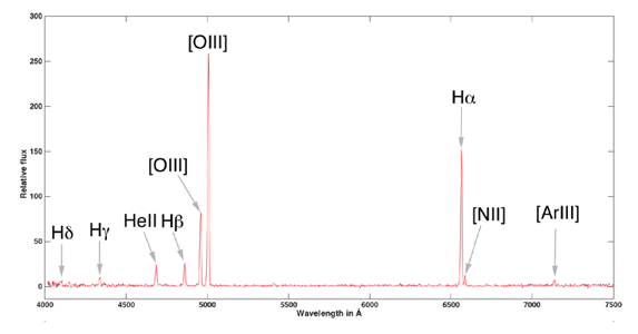
A typical planetary nebula spectrum obtained with a LISA
Methodology
Once you’ve determined your target candidate, you need a field chart made with free software available online such as Aladin.
We enter the coordinates of the target in Aladin and we can see the chart of the target whose magnitude is very weak (magnitude generally greater than 16). The image of the autoguiding sensor field can be overlaid on the image produced by Aladin.
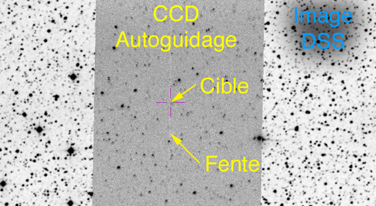
Example of overlaying the autoguiding sensor field with the DSS image in Aladin
It’s not uncommon that the target doesn’t stand out on the autoguiding sensor because of the weak source of light. We will position the slit of the spectrograph depending on the surrounding stars. Save an image of the autoguiding sensor field on your PC in order to attach it to the future observation report of this target. The autoguiding will be done on a bright star close to the target while you check that the slit is on the target. Once centered, we start the autoguiding then we go to the acquisitions of the spectra :
- 1- Produce a first image with a unit exposure time of 900 to 1200 seconds. If there is no apparent signal, drop this target. This phase is delicate, an adjustment of the thresholds is sometimes necessary to try to perceive the signal. If nebular lines appear, acquisition can continue. The image below shows the appearance of a raw unit spectrum of a rather punctual NP candidate.
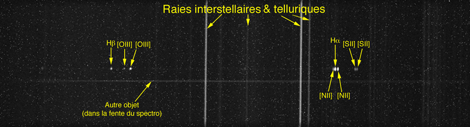
Example of a raw spectrum as it appears on the PC screen during acquisitions by finely tuning the display thresholds.
- 2- Take n poses of 900 seconds. n depends on the appearance of the unit spectrum and can vary from 3 to 12 depending on the targets. The goal is to increase the signal to noise ratio in order to highlight the main emission lines.
- 3- Take a spectrum of a calibration lamp (Neon), without modifying the position of the spectrograph or the telescope.
- 4- To perfectly calibrate the spectrum, it’s necessary to take the spectrum of a reference star (A or B) close to the target and at the same height in the sky. For that we will use the excel spreadsheet offered by François Teyssier and available here. Pointing the reference star : take a series of 7 to 9 unit spectra whose exposure times depends on the magnitude of the star (between 2 and 5 seconds most of the time because of the brightness).
- 5- Take a spectrum of the calibration lamp (Neon), without modifying the position of the spectrograph and/or the telescope.
- 6- Switch to the next target. Note that each spectrum is made exactly at the same x and y coordinates of the slit which allows for better accuracy during processing.
- 7- At the end of the acquisitions, a series of 21 to 33 images use a tungsten lamp for the flats.
Spectrum processing
The processing will be carried out with ISIS which makes it possible to choose the right treatment zone of the spectrum.
The reference star is first processed to calculate the instrumental and atmospheric effect response at the time of observation. Once the processing is done, the resulting spectrum is compared to a generic spectrum of a star of the same type in the ISIS database. The resulting Planck profile is verified.
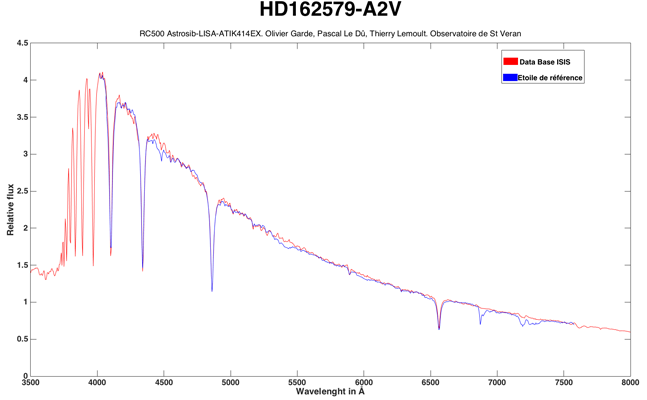
The example above shows the result with a A2V star. The red curve is the reference curve of the ISIS database and the blue curve of the reference star obtained with the spectrograph. The two curves must be superimposed.
The target is then processed. The job is now to select the area of interest within the image, from which the final spectrum of the object will be calculated. Two areas containing only the sky background need to be identified in order to be subtracted from the area of interest containing the object’s signal. The goal here is to eliminate all lines of light, interstellar pollution as well as the Earth’s atmosphere or even another nebula that could be in the same line of sight as the NP. Only the signal related to the object must be taken into account.
This work is relatively easy in the case of a punctual NP. It becomes harder for a diffuse NP because the different zones to be determined are difficult to identify. Often, several tests are necessary.
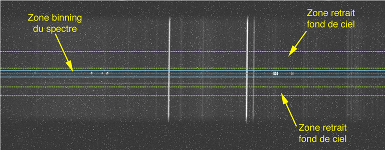
The example above shows the treatment performed on a candidate NP punctual, so “easy”. The zone delimited in blue contains the area of the spectrum of the NP that will be treated. The height is adjusted to contain the entire signal of the NP. Do not hesitate to push the thresholds of the histogram for visualization. It is in this zone that the spectrum is calculated (by adding the pixels of each column of the zone).
The two green areas are selected at the top and bottom of the spectrum. They do not have star spectra that could disturb the measurements in the area of interest. These sky-bottom areas are positioned closest to the area of the NP spectrum calculation.
Once the treatment is done, we finally obtain a spectrum that can look like this :
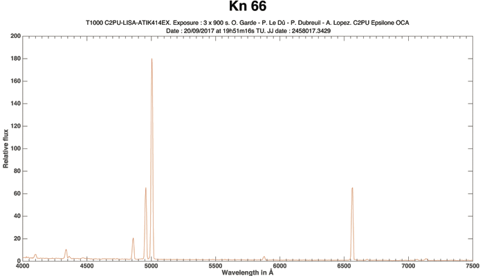
Example of the KN 66 candidate : we can see the various nebular lines
Spectrum analysis
We will try to analyze the spectra obtained to determine if it is indeed a planetary nebula and not another object such as a proto-star, a nova, a galaxy or other object that does not have the spectral signature of a planetary nebula like the example below which is actually a Seyfert galaxy not yet listed.
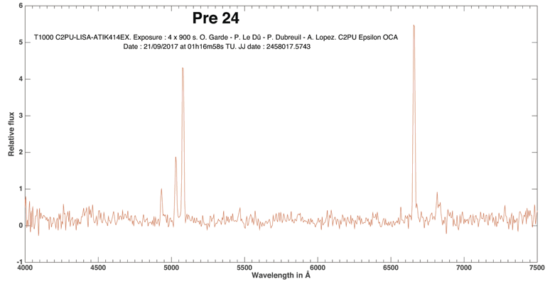
Pre24 spectrum showing nebular lines but strongly shifted in the red. We can also calculate its redshift z which in this case is z = 0.014 is a velocity of more than 4300 km/s. We can therefore exclude this candidate who is not an NP.
Publication of results
The collection of spectral data is done by Pascal Le Dû who gathers the various spectra obtained to send them to Quentin Parker and his team of the University of Hong Kong who maintains the HASH planetary nebula database :
You can download a report form template here and send it to ledu at shom dot fr with all spectra data files (.fits, .dat, .log et .xml)
Regularly the astronomical database is updated of the latest confirmations where the objects pass from the stage “Possible Planetary Nebula” to the stage of “Planetary Nebula” in full share as on the example below :
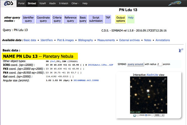
Example of a Nebula that has been confirmed in spectroscopy
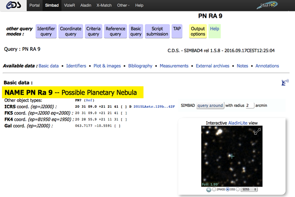
Example of a target that has not been confirmed yet
References :
-
Planetary Nebula Confirmation Mission Report to St Veran Observatory : http://o.garde.free.fr/RapportMissionCALAI-2016BD.pdf
-
Planetary Nebula Confirmation Mission Report to the OCA on the Calern observatory : http://o.garde.free.fr/RapportMissionCalern2017.pdf
- The Pascal Le Dû website : http://www.cielocean.fr
-
The APN VII congress poster in Hong Kong : http://www.cielocean.fr/uploads/images/FichiersPDF/Poster_APN%20VII%20v1-1.pdf
-
The issues of the french magazine l’Astronomie relating the confirmations of planetary nebulae : # 91 February 2016, # 102 February 2017 and # 114 March 2018 : https://www.saf-lastronomie.com/revue/
- The french magazine Ciel et Espace # 558 March/April 2018 : https://boutique.cieletespace.fr/liseuse/preview/558/view.html#!/avedocument0/pdf/1/1/1
- Discovery of new faint northern galactic PN : http://www.cielocean.fr/uploads/images/FichiersPDF/RMxAA..48-2_aacker.pdf
- Article in french about Pascal Le Dû observations : http://www.cielocean.fr/uploads/images/FichiersPDF/ASM87_SpectroGa1.pdf