Study of a spectroscopic binary with amateur setup

By David Antao

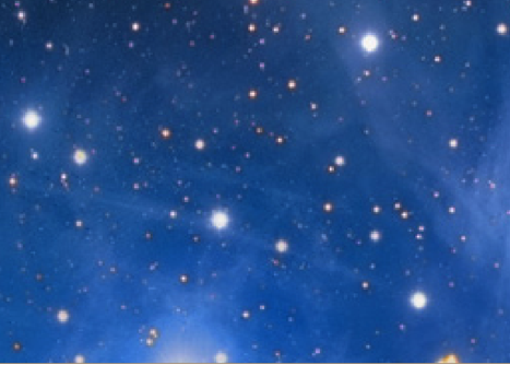
Photo credit : Vivien Pic

In this article, I will try to show you that amateur astronomers can achieve remarkable results in the astrophysical study of the stellar world. For some years now, we have had powerful tools at our fingertips. We can, thanks to them, have access to the dynamics of the sky and to carry out our own studies, either for our greatest pleasure, or also to participate, at our modest level, in the progress of science. The ideal is to combine the two, which I could do in the study of this spectroscopic binary star. Indeed, many collaborations between professional astrophysicists and amateur astronomers have started with encouraging results.

During a meeting between professionals and amateurs, was born my collaboration with David Valls-Gabaud, astrophysicist at Paris Meudon observatory. He suggested me to follow a spectroscopic binary. I was finally able to combine the pleasure of amateur observation with the utility for research! And for an amateur astronomer it’s great!

What is a spectroscopic binary?

It’s a pair of stars linked by gravity that revolve around each other. The closer they are, the shorter their period, the faster they spin around each other and the less they can be separated in a telescope, until they can no longer be used even by the largest telescopes today. What is great is that we will be able, in these cases, use a spectroscope and thanks to the Doppler-Fizeau effect, we will see the 2 stars turn around each other. We have access to the sky in motion!

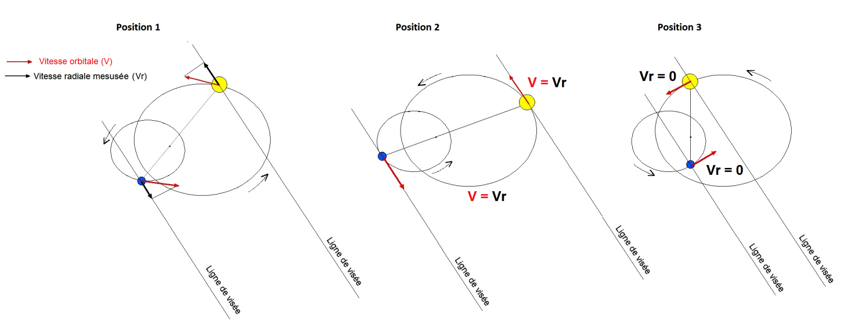
Composition of the orbital binary velocities seen from the Earth.
The red arrow symbolizes the proper speeds of the stars. On the other hand, only the projection of these velocity on our axis of observation, symbolized by the black arrow, is accessible to us. It’s called radial velocity. This velocity is maximum when the stars are in position 2 and minimal or even zero when they are in position 3.

The target was HD23642, a star in the Pleiades of magnitude 6.9 and A0V spectral type. This magnitude is low for the LhiresIII 2400 gr/mm and a 250 mm telescope. It was necessary to choose to carry the study on the line H beta, because the flux in this wavelength is superior to H alpha for the hot stars. The unit exposure was 20 minutes.

This couple of stars has a period of about 2.5 days. It took me several nights to cover almost the entire period. This led to 319 high resolution spectra of which only 245 were exploitable. This low efficiency is due to some disturbances (clouds, wind, humidity too strong …) that degrades the signal-to-noise ratio and the spectrum is no longer usable. This represents a total of about 122 hours of observation to capture 91% of the revolution. This is also the strength and usefulness of amateur astronomers: having a lot of telescope time to be able to devote to a long background work.

My first spectra

Here are 3 spectra at different times of the orbital period. It is easy to see that the profile of the H beta line changes with time.

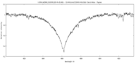
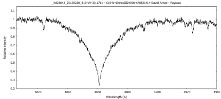
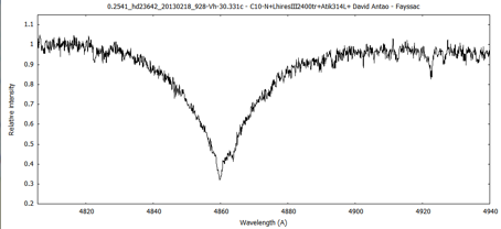
What is important to understand is that our spectrum is the addition of the light of 2 stars. Depending on the position of the stars in their orbit, seen from Earth, a star moves away from us, while the other approaches. So when we integrate the Doppler-Fizeau effect, the H beta line of the approaching star will be shifted to the blue (that is to say towards the left part of the spectrum) and the one that moves away will be shifted towards the red (that is to say towards the right part of the spectrum).

Decomposition of the observed spectrum

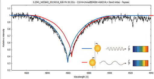
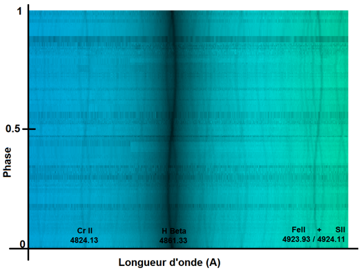
We will have the impression that the line is split. This applies to H beta line, but also for all other lines, except the atmospheric lines, as can be seen on the stack of spectra as a function of the phase.

Classification of 2D spectra according to the phase

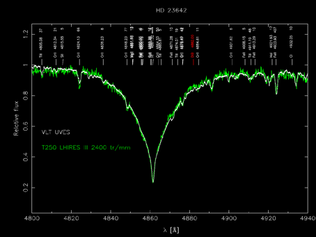
It’s very good think to make all these amateur spectra, but what quality can they have? After asking the question to David Valls-Gabaud, he replied that it was very good, but the doubt is still present … until the famous evening before going to bed around 11 pm, I look at one last times my emails. Here is an email from David: “Here is a spectrum of HD23642 acquired by the UVES instrument of the VLT”. What was my surprise when I opened the attachment …. It was one of the greatest emotions of my life as an astronomer. Can not find sleep before late at night! My spectra are superbly overlapping with those of the VLT, but of course, I am far from competing with the VLT with my 250mm telescope. To compare, the VLT realized in a single exposure a spectrum over the entire visible range and even a little beyond. The exposure time on the UVES instrument of the VLT was 110 seconds, against 1200 seconds for me, only around the H beta line. But still, the result is impressive!

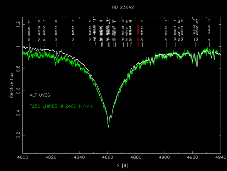
Superposition of amateur spectrum with a spectrum of VLT

Note on the second superposition, that the blue part of the amateur spectrum (left side of the spectral line) is slightly less intense. This is due to a bad correction of the atmosphere effect. On the other hand, it does not affect the shape, the position of the lines, and therefore neither the radial velocities.

Once all the observations made and the spectra sent to the professional astrophysicist, I wanted to go further than the observations. I joined at that time with David Brégou, amateur astronomer like me and fascinated by the science side of amateur astronomy.

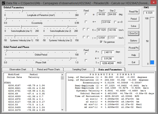
It was first necessary to extract the radial velocities of the two components on all spectra. Then with the software “Spectroscopic Binary Solver” Delwin Owen Johnson, published in “The Journal of Astronomical Data” of November 9, 2004, it was possible to calculate the physical parameters of this pair of stars.

This software is available HERE

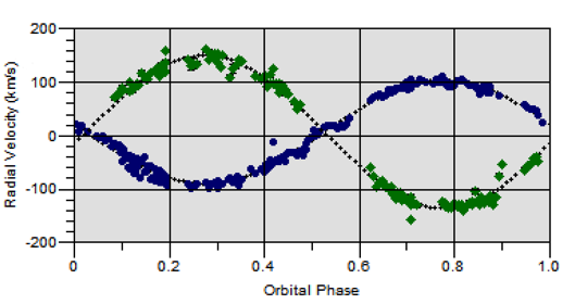
And there, it was a second great emotion when after a few clicks the cloud of points arranged according to the date, is organized in two beautiful sinusoids according to the phase.

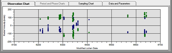
Before switching to SBS software

The blue dots are the measurements of the radial velocities of the first star and the greens are those of the second star, classified according to the date of acquisition.

After switching to SBS software

All points are classified according to the calculated phase.

The physical parameters of the binary system were calculated by the software

• Period 2.46119 days
• Maximum radial velocity of the two stars K1 = 97.10Km/s and K2= 143.11 Km/s
• Eccentricity of the orbits e=0.011
• Proper motion of the binary system compared to the sun : 6.9 Km/s, which means that HD23642 away from sun, or I prefer to say that the Sun is moving away from this couple of stars from 6.9 Km/s.
• And finally the two semi major axes and the masses of each of the stars according to the sin i, or the inclination of the orbits with respect to our line of sight:

– semi major axes of the most massive star a1.sin i = 3 286 106 Km ^{+/- 28 700}

– semi major axes of the least massive star a2.sin i = 4 843 106 Km ^{+/- 31 400}

– Mass of the biggest star m1.sin 3i = 2.106 ^{+/- 0.0137} solar mass

– Mass of the smallest star m2.sin 3i = 1.427 ^{+/- 0.0125}7 solar mass

SBS results

It’s exciting that from the study of radial velocities we can get all this information on the physics of a couple of stars.
THANK YOU KEPLER!

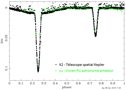
Being president of an astronomy club in the Tarn http://www.astrosurf.com/apam/ Of course, I did a preview of my work to my friends from the Astronomy Association Montredonnaise of Photography, A.P.A.M. This gave some people the desire to go further and especially with additional measurements in photometry, by Vivien Pic. This was possible because this spectrometric binary is also an eclipse binary. In spectroscopy we will be able to make the measurements above, but the inclination is inaccessible to us; precisely photometry will fill this gap. And in the end, we can go even further in the study of this pair of stars, and even estimate its distance and suddenly, that of the cluster of which it is a part.

Vivien followed this star with a 100mm telescope and the results are well compatible with those of the Kepler spacecraft! This precision is remarkable!

The assessment of measures

With photometry

Period : 2.4611 ^{+/- 0.7e-6} jours
Eccentricity : 0.0 ^{+/- 0.005}
Tilt (°) : 77.2 ^{+/- 0.15}
#1 star radius : 1.831 ^{+/- 0.04} Rsol
#2 star radius : 1.608 ^{+/- 0.05} Rsol

And the final results :

#1 star radius : 1.831 ^{+/- 0.04} solar radius
#2 star radius : 1.608 ^{+/- 0.05} solar radius
#1 star mass : 2.260 ^{+/- 0.030} Solar mass
#2 star mass : 1.517 ^{+/- 0.025} Solar mass
Semi-major axis a1 : 3.338.106 ^{+/- 2.89e+4} Km
Semi-major axis a2 : 4.973.106 ^{+/- 3.16 e+4} Km

What is most extraordinary that they are distant from each other by only a little more than 8 million km or about 0.05 astronomical unit (AU), it’s 7 times closer than the Sun-Mercury distance.

And finally, we calculated the distance thanks to the distance module

With :
m = apparent magnitude
M = absolute magnitude
D = distance in Parsec

We fin around 150pc (light-years), calculated with an interstellar extinction estimated at 0.5 mag. The distance measured by Gaia is 134 +/- 6 pc. The difference is justified by the fact that interstellar extinction is difficult to estimate, especially in this region.

That’s our amateur study. David Valls Gabaud has not published his results yet as I write these few lines. It’s a long time, but we are astronomers and we know how to be patient. This is good for us, because like that we were not influenced for our calculations. When the publication comes out, we will be able to see how good our study is and identify any gaps so we can better understand them next time. One thing is certain, our personal knowledge have progressed well during these manips for our greatest pleasure !!!

In February 2016 another publication appeared on this star.

Here are the comparisons

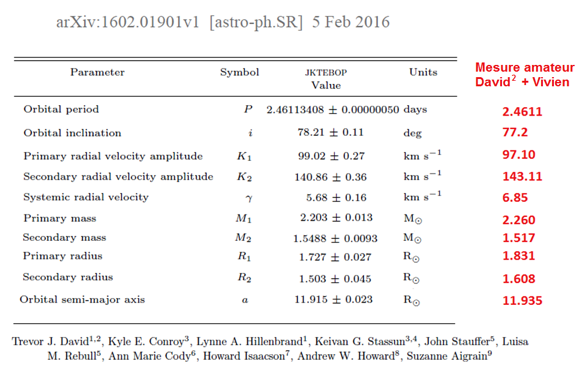
David Valls-Gabaud, tells us results better than 1% see publication SF2A : ASTROPHYSICS OF VERY HIGH PRECISION BY AMATEURS: THE CASE OF A SPECTROSCOPIC BINARY ECLIPSANTE. SF2A 2018

https://ui.adsabs.harvard.edu/abs/2018sf2a.conf..403A/abstract

and the PDF here : http://sf2a.eu/proceedings/2018/2018sf2a.conf..0403a.pdf

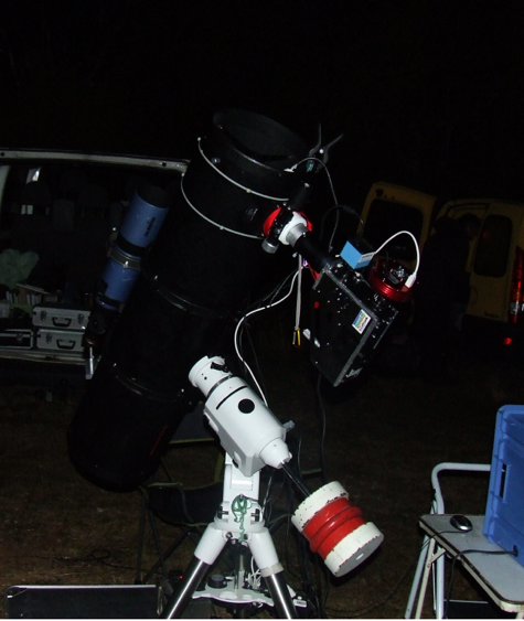
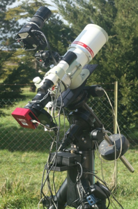
Material used to perform spectroscopic observations: Newton telescope 250mm aperture on EQ6 equatorial mount, Spectro LhiresIII 2400 gr/mm focus on Hbeta line and a CCD Atik 314L+